Of all the many programming languages, none has quite caught my attention like the “Iversonian” programming languages, that is, languages like APL, Shakti, Ivy, BQN and J - the subject of this blog post.

One misconception is that languages like J are in the same caliber as Brain F**k and other esoteric or golfing languages which are mostly for recreational programming. Languages like J however were designed to be a replacement to traditional maths notation - an interface for thinking or a tool of thought as their inventor Kenneth E. Iverson called them in his Turing Award lecture.

In this blog post I am going to introduce the J programming language by using it as a “tool of thought” to explain the 1 dimensional random walk.

To try out the code yourself you will have to install the J interpreter. The easiest way to get it working on Mac is through running the brew formula brew install --cask j. For other platforms, see the installation instructions.

First, a random walk in 5 lines. #

The 1 dimensional random walk is a toy model used in finance for creating what may look like stock market prices. In it’s simplest form, a 1 dimensional random walk consists of;

• Several steps (a list of values), and at each step (for each value) it is either up (indicated by +1) or down (indicated by -1).
• Note that the value of each step -1 or +1 is chosen at random. Hence the term ‘random walk’. So a random walk is basically a list of -1 and +1 generated at random.
• To attain the ‘synthetic price’ or what looks like stock prices, we simply compute the running sum of this list of random -1 and +1 integers.

The entire toy model of prices we described above is created using the J code below. Let me describe how.

load 'plot' NB. Import the utility for plotting  charts
indices     =: ? 100#2          NB. Generate indices
walks       =: indices { _1 1   NB. Use indices to create list of -1 & +1 integers
running_sum =: +/\ walks        NB. Compute synthetic price
plot running_sum                NB. Plot the running sum

Generating indices. #

An index refers to the position of an item in a list. For example, the list 1 2 3 4 has the indices 0 for 1, 2, 3, with the index 0 referring to 1, the index 1 referring to 2, the index 2 referring to 3 and the index 3 referring to 4.

Line 2, indices =: ? 100#2 generates indices as follows. The # symbol takes in two values 2 and 100 and what it does is that it “copies” 2 into an list 100 times. For example 5#1 copies 1 five times to give 1 1 1 1 1. So 100#2 returns 2 2 2 2 2 2 2 2 2 2 ... 2 up to the 100’th 2.

The ? symbol generates random numbers, you can think of it as rolling a dice. For example, ? 5 may randomly return 0, 1, 2, 3 or 4. So ? 5 can be read as “generate a random number below 5”, 0 is included since the values ? generates are always greater than or equal to 0.

And finally to generate a list of random numbers, we simply give ? a list of numbers for example ? 3 3 3 3 3 may generate 1 1 0 2 2 i.e 5 random numbers under 3. Recall that in line 2, 100#2 generates a list of one hundred 2’s. ? then takes the list of one hundred 2’s and for each 2 it generates a random number less than 2 i.e 0 or 1.

? 100#2 can be read as “generate a list one hundred 2’s and for each item in the list, generate a random integer less that 2”. This will return a random list of 100 items made up of exclusively 1’s and 0’s looking like 0 0 1 1 0 0 1 1 1 0 0 1 0 1 0 1 1 0 1 0 1 1 0 1 .... We then store this in a variable called indices using =:

This is what we shall use as our indices.

Use indices to create list of -1 & +1 integers. #

In line 3, we use our list of 0’s and 1’s as indices to generate a random walk (random list made up of -1’s & +1’s). To do this, we use the symbol { in indices { _1 1 that takes in two sets of values, first is the variable indices which is a list of randomly generated 1’s & 0’s. On the other side of { is _1 1, which represent the directions of our random walk _1 for -1 (down) and 1 for +1 or (up).

What { does is that it “pulls” items from a list given an index. The list _1 1 has the indices 0 for _1 and 1 for 1, recall that an index refers to the position of an item in the list. So the statement 0 { _1 1 would return _1 and 1 { _1 1 returns 1 from the list.

A list of indices would also return a list of items, for instance 1 0 0 1 { _1 1 would return 1 _1 _1 1. Which is similar to what indices { _1 1 is doing. Since indices is a list of random one hundred 1’s and 0’s it will also randomly pull out a list of _1 and 1 thus giving us a list like _1 _1 1 1 _1 _1 _1 _1 _1 _1 1 _1 ... up to the one hundredth index. Which is the random walk of 100 steps.

We also store this list into a variable walks using =:.

Compute the synthetic prices. #

In line 4 we use +/\ the running sum of the random walk. For example +/\ 1 1 1 1 1 1 1 computes the running sum of seven 1’s, which gives us 1 2 3 4 5 6 7. Which is exactly what we do with +/\ walks.

Since walks is made up of randomly generated _1 and 1, it’s running sum will equally fluctuate up and down. The running sum of 1 _1 1 _1 _1 _1 1 1 1 _1 _1 will look like 1 0 1 0 _1 _2 _1 0 1 0 _1

The running sum (synthetic price) +/\ walks is then stored inside the variable running_sum with =:

A random walk in 2 lines. #

This post was supposed how to create a random walk in 2 lines of J. So below is the exact code above refactored to run in two lines.

load 'plot'              NB. Import the plot library
plot +/\ (?100#2) { _1 1 NB. Plot synthetic price/ random walk

Adjusting step size #

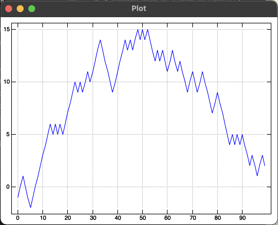
100 denotes the number of steps the random walk takes. The more the steps the closer to actual stock prices the plot will look like.

Random Walk of 100 steps #

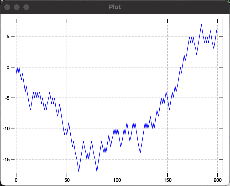
Random Walk of 200 steps #

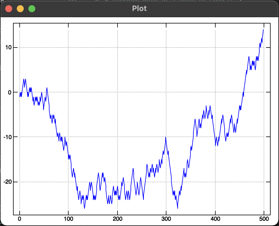
Random Walk of 500 steps #

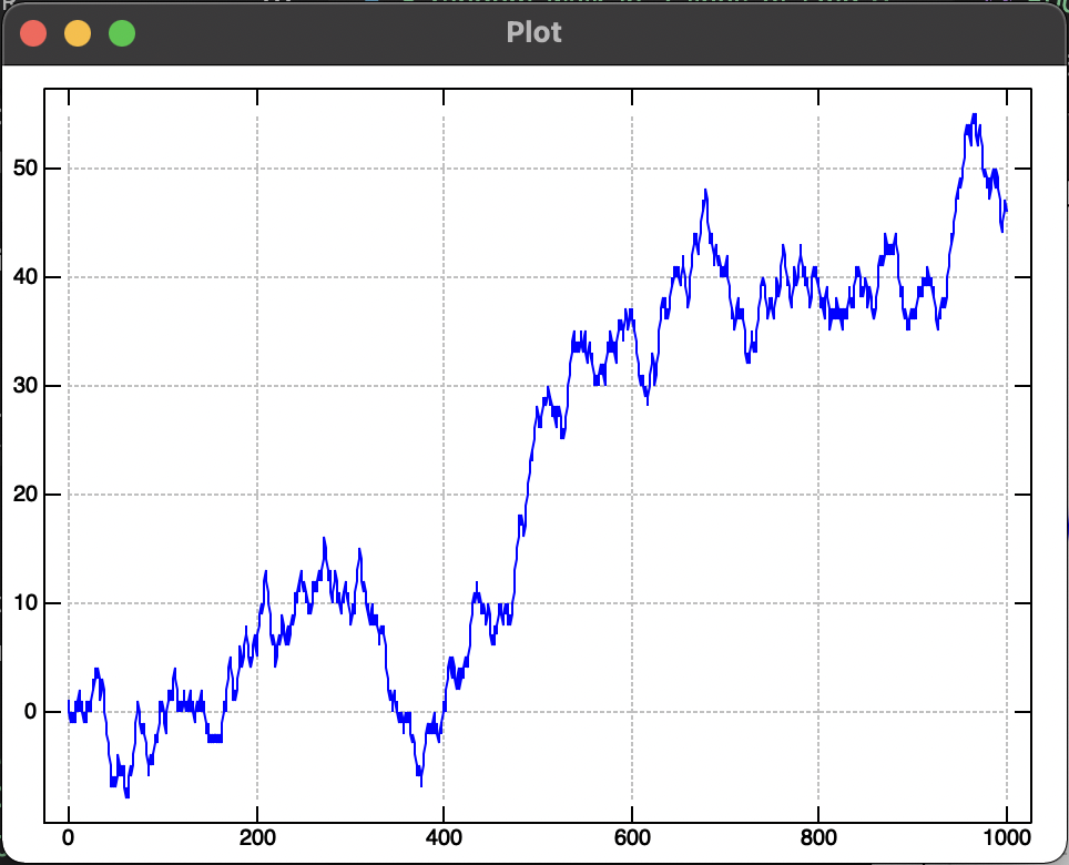
Random Walk of 1,000 steps #

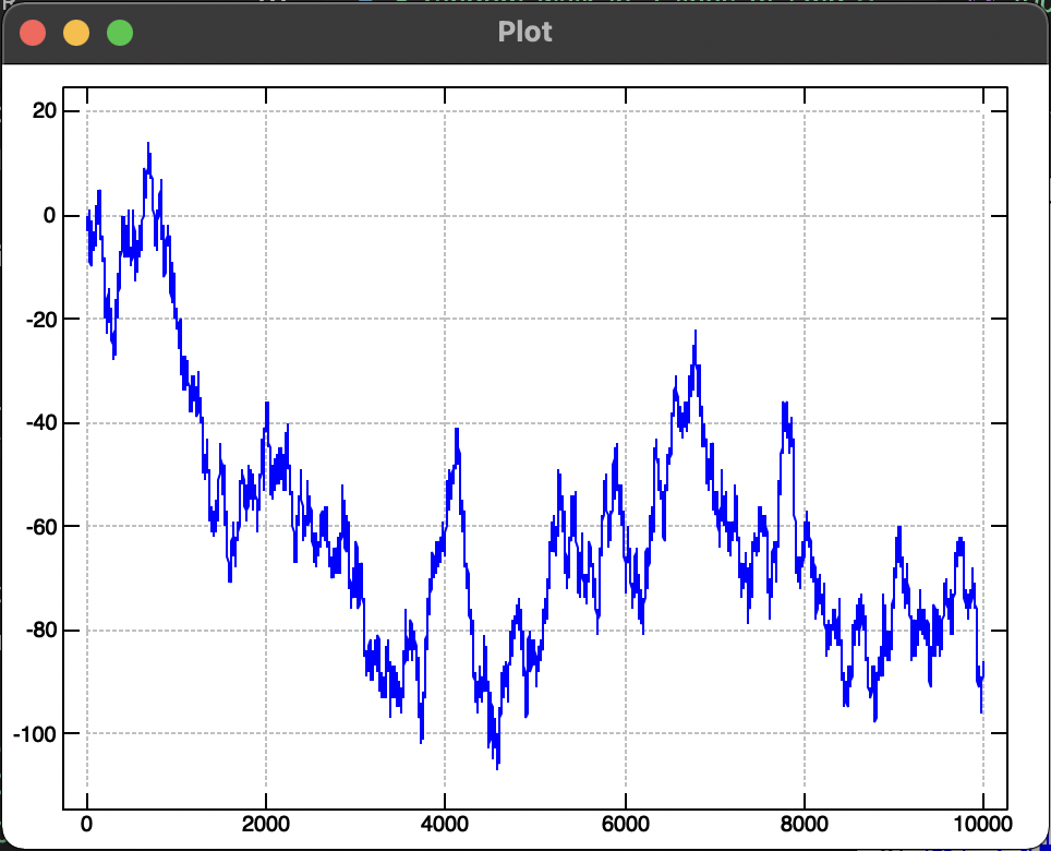
Random Walk of 10,000 steps #