3C. Graphs versus
function tables
3D. Notes
A table of the
function
"twenty-five minus
the square", or
"twenty-five with
minus
on the square" for
each item of the
argument
However, the
characteristics of
the
function can be
seen more easily
in a graph of
the function,
produced by
plotting each
column
of the table as
follows: starting
at
an arbitrary point
on a sheet of
squared
paper measure a
distance
Graphs can be
produced
quickly and
accurately by the
computer as
follows:
Plots of
polynomial
functions may show
further
interesting
characteristics.
For
example, study the
plot of the
following
function,
use
Remarks:
The result of
To anyone familiar
with the functions
sine and cosine of
trigonometry, it
may be
evident that the
functions
Moreover, the
cosine and sine of
a given angle are
sometimes defined
as the coordinates
of a
point on the unit
circle of radius
1, located
at the given angle
(that is, the arc
length
along the
circumference). It
should therefore
come as no
surprise that the
plot of
The expression
In addition to
providing an
overall view of
a function, its
graph shows the
local
behaviour, the
slopes of the
individual
segments
reflecting its
local rates of
growth
and decay.
Moreover, the
graph provides
a direct view of
the area under it,
a result
of considerable
significance.
This will be
illustrated by a
plot of a
semi-circle. The
function
The function
The last result is
the approximate
area
of the complete
circle, and is
therefore an
approximation to
the constant
Tables of
functions that
apply pairwise
to their arguments
can, however,
provide
similar insights.
Moreover, they can
provide
other information
(such as the rate
of
change of the rate
of change) not
readily
grasped from a
graph.
To this end we
will define a
pairwise
operator
Pairwise relations
such as
Any reader puzzled
by certain
notations
(such as the
double use of
4B.
Notes
Polynomials
are
important
for a
number
of
reasons:
*
Because
of the
wide
choice
of
coefficients
available,
polynomials
can be
defined
to
approximate
most
functions
of
practical
interest.
* As
already
illustrated
for
sums,
products,
and
composition
of
polynomials,
they
are
closed
under
a
number
of
important
functions,
in the
sense
that
the
resulting
function
is
again
a
polynomial.
These
include:
In
most
of
these
cases,
the
Taylor
operator
can be
used
to
obtain
the
coefficients
of the
resulting
polynomial.
With
increasing
use of
computer
experimentation,
it
becomes
important
to
learn
to
use
the
available
tools.
In
particular:
5B.
Truncated
power
series
5C.
Notes
On
the
other
hand,
the
power
series:
As
illustrated
by
the
last
column,
these
truncated
power
series
are
approximations
to
the
trigonometric
sine
function
(on
radian
arguments).
Moreover,
the
Taylor
operator
However,
it
was
possible
to
confine
that
discussion
to
rather
elementary
ideas,
whereas
a
meaningful
discussion
of
the
uses
of
power
series
would
quickly
lead
to
more
advanced
and
less
familiar
mathematical
notions
outside
the
experience
of
many
readers.
The
same
is
true
of
many
topics
(such
as
the
derivative,
symbolic
logic,
sets,
and
permutations),
and
we
will
leave
the
reader
to
observe
the
importance
of
topics
as
they
are
exploited
in
later
work.
In
other
words,
some
faith
is
expected
of
the
reader
"
a
belief
that
topics
will
be
introduced
only
if
they
are
both
important
and
interesting.
6B.
Derivatives
of
polynomials
6C.
Taylor
coefficients
6D.
Notes
Considered
as
a
sample
of
points
on
a
continuous
graph
of
the
function
(using
an
infinite
number
of
points),
these
sloping
lines
are
secants
(cutting
lines)
to
the
continuous
curve,
and
the
slope
at
a
point
is
the
tangent
(touching
line)
to
the
curve,
which
may
be
approximated
by
a
secant
with
a
small
interval.
The
expression
Multiplication
of
the
sums
gives
the
square
of
Similar
calculations
for
the
product
This
is
all
embodied
in
the
calculation
Note
that
the
zero
value
of
the
graph
of
the
derivative
occurs
at
the
argument
value
for
which
the
original
function
reaches
its
low
point,
that
is,
where
its
graph
is
horizontal.
The
phrase
derivative
of
In
this
chapter
we
have
skirted
the
issue
by
confining
attention
to
polynomial
functions,
for
which
the
limit
of
the
secant
slope
is
easily
obtained.
We
will,
however,
extend
these
results
to
the
many
important
functions
that
can
be
approximated
by
the
power
series
(themselves
polynomials)
that
were
discussed
in
Chapter
5.
Can
we
be
certain
that
the
derivative
of
a
polynomial
approximation
to
a
function
7B.
The
name
"exponential"
The
simplest
case
is
where
the
rate
of
growth
is
equal
to
the
size
--
this
is
described
by
the
exponential
function,
denoted
here
by
Since
a
polynomial
may
be
found
that
can
approximate
almost
any
function,
it
should
be
possible
to
find
one
that
approximates
the
exponential.
Consider
the
following:
In
the
dyadic
use
of
the
symbol
8B.
Harmonics
8C.
Decay
If
Moreover,
the
acceleration
is
caused
by
the
"restoring
force"
exerted
by
the
spring,
which
is
proportional
to
its
extension
as
measured
by
the
position
In
the
simplest
case
9B.
Equations
9C.
The
method
of
false
position
9D.
Newton"s
method
9E.
Roots
of
Polynomials
9F.
Logarithms
The
need
for
inverse
functions
arises
frequently.
For
example,
the
heat
produced
by
an
electric
heater
may
be
given
by
the
function
The
function
The
element
of
Although
Newton"s
method
converged
rather
rapidly
for
the
function
Nevertheless,
the
function
The
logarithm
is
discussed
further
in
Chapter
20.
10B.
Word
formation
10C.
Parsing
10D.
Conventional
mathematical
Notation
Formal
grammar
becomes
particularly
important
in
writing,
where
the
reader
has
no
recourse
to
interjected
questions,
but
must
extract
meaning
from
the
text
alone.
Similar
considerations
apply
in
mathematics.
Although
the
Hogben
remarks
cited
in
our
preface
emphasize
the
importance
of
language
and
grammar,
we
have
introduced
the
grammar
of
our
language
J
only
informally,
allowing
us
to
concentrate
on
the
mathematical
notions
it
has
been
used
to
convey.
This
informal
approach
has
been
made
tolerable
by
limiting
the
writing
required
of
a
student
in
Exercises
to
imitation
of
expressions
already
used,
and
by
providing
guidance
through
conversation
with
the
computer,
a
native
speaker
of
the
language.
This
chapter
will
address
the
formal
grammar
of
J,
and
will
also
comment
on
the
more
loosely
structured
grammar
of
conventional
mathematical
notation.
In
a
written
English
sentence
this
process
is
so
simple
as
to
go
unnoticed,
although
the
separation
by
spaces
is
somewhat
complicated
by
things
such
as
hyphens
and
apostrophes.
In
oral
communication
it
is
also
unnoticed,
not
because
the
breaking
of
a
continuous
stream
of
sound
into
words
is
simple,
but
because
(except
in
the
case
of
a
foreign
language)
it
is
so
deeply
ingrained.
In
the
case
of
J
the
word
formation
requires
some
attention,
although
it
is
simple
enough
to
have
been
thus
far
treated
informally
by
example.
The
computer
provides
a
word-formation
function
that
may
be
applied
to
a
sentence
enclosed
in
quotes.
Thus:
Alternative
spellings
for
the
national
use
characters
(which
differ
from
country
to
country)
are
discussed
under
Alphabet
( Numbers
are
denoted
by
digits,
the
underbar
(for
negative
signs
and
for
infinity
and
minus
infinity
--
when
used
alone
or
in
pairs),
the
period
(used
for
decimal
points
and
necessarily
preceded
by
one
or
more
digits),
the
letter
A
numeric
list
or
vector
is
denoted
by
a
list
of
numbers
separated
by
spaces.
A
list
of
ASCII
characters
is
denoted
by
the
list
enclosed
in
single
quotes,
a
pair
of
adjacent
single
quotes
signifying
the
quote
itself:
Names
(used
for
pronouns
and
other
surrogates,
and
assigned
referents
by
the
copula,
as
in
A
primitive
or
primary
may
be
denoted
by
a
single
graphic
(such
as
A
sentence
is
evaluated
by
executing
its
phrases
in
a
sequence
determined
by
the
parsing
rules
of
the
language.
For
example,
in
the
sentence
Moreover,
the
left
argument
of
an
adverb
or
conjunction
is
the
entire
verb
phrase
that
precedes
it.
Thus,
in
the
phrase
One
important
consequence
of
these
rules
is
that
in
an
unparenthesized
expression
the
right
argument
of
any
verb
is
the
result
of
the
entire
phrase
to
its
right.
The
sentence
Parsing
proceeds
by
moving
successive
elements
(or
their
values
except
in
the
case
of
proverbs
and
names
immediately
to
the
left
of
a
copula)
from
the
tail
end
of
a
queue
(initially
the
original
sentence
prefixed
by
a
left
marker
")
to
the
top
of
a
stack,
and
eventually
executing
some
eligible
portion
of
the
stack
and
replacing
it
by
the
result
of
the
execution.
For
example,
if
Parsing
can
be
observed
using
the
trace
conjunction
The
classes
of
the
first
four
elements
of
the
stack
are
compared
with
the
first
four
columns
of
the
table,
and
the
first
row
that
agrees
in
all
four
columns
is
selected.
The
bold
italic
elements
in
the
row
are
then
subjected
to
the
action
shown
in
the
final
column,
and
are
replaced
by
its
result.
If
no
row
is
satisfied,
the
next
element
is
transferred
from
the
queue:
It
includes
a
discussion
of
the
learnability
of
mathematical
notation
as
compared
with
other
specialized
notations
and
with
native
languages,
as
well
as
the
importance
of
such
learnability.
SOME
HISTORICAL
VIEWS
ON
NOTATION
Mathematicians
have
often
noted
the
power
and
importance
of
notation.
In
Part
IV
of
his
two-volume
A
History
of
Mathematical
Notations
[3],
Florian
Cajori
offers
the
following
examples:
Nothing
in
the
history
of
mathematics
is
to
me
so
surprising
or
impressive
as
the
power
it
has
gained
by
its
notation
or
language
...
But
in
Napier"s
time,
when
there
was
practically
no
notation,
his
discovery
or
invention
[of
logarithms]
was
accomplished
by
mind
alone,
without
any
aid
from
symbols.
J.W.L.
Glaisher
Some
symbols,
like
an,
...,
log
n,
that
were
used
originally
for
only
positive
integral
values
of
n
stimulated
intellectual
experimentation
when
n
is
fractional,
negative,
or
complex,
which
led
to
vital
extensions
of
ideas.
F.
Cajori
The
quantity
of
meaning
compressed
into
small
space
by
algebraic
signs,
is
another
circumstance
that
facilitates
the
reasonings
we
are
accustomed
to
carry
on
by
their
aid.
Charles
Babbage
Symbols
which
initially
appear
to
have
no
meaning
whatever,
acquire
gradually,
after
subjection
to
what
might
be
called
experimenting,
a
lucid
and
precise
significance.
E.
Mach
In
Sections
740
ff,
Cajori
laments
the
lack
of
standardization
of
mathematical
notation
in
the
following
excerpts:
"740
Uniformity
of
mathematical
notations
has
been
a
dream
of
many
mathematicians
...
"741
The
admonition
of
history
is
clearly
that
the
chance,
haphazard
procedure
of
the
past
will
not
lead
to
uniformity.
"746
In
this
book
we
have
advanced
many
other
instances
of
"muddling
along"
through
decades,
without
endeavor
on
the
part
of
mathematicians
to
get
together
and
agree
on
a
common
sign
language.
"748
In
the
light
of
the
teaching
of
history
it
is
clear
that
new
forces
must
be
brought
into
action
in
order
to
safeguard
the
future
against
the
play
of
blind
chance.
...
We
believe
that
this
new
agency
will
be
organization
and
co-operation.
To
be
sure,
the
experience
of
the
past
in
this
direction
is
not
altogether
reassuring.
However,
in
William
Oughtred:
A
Great
Seventeenth-Century
Teacher
of
Mathematics
[4],
Cajori
touches
on
a
quite
different
agency
that
bears
upon
the
development
and
teaching
of
mathematics
--
the
mathematical
instrument.
On
page
88
we
have:
PROGRAMMING
LANGUAGES
Early
computers
provided
a
small
set
of
operations
such
as
addition
and
multiplication,
and
were
controlled
by
programs
specifying
sequences
of
these
operations.
For
example,
on
the
Harvard
Mark
IV
[5],
the
program:
Programs
were
later
developed
to
translate
from
languages
more
congenial
to
mathematicians
into
equivalent
machine
language
programs
for
subsequent
execution.
For
example,
in
BASIC,
a
language
largely
derived
from
FORTRAN
(Formula
Translator)
[6],
one
might
write:
Moreover,
many
have
moved
to
Computer
Science,
unwittingly
following
the
advice
of
Newton,
as
expressed
in
the
following
excerpt
from
page
95
of
Cajori
[4]:
The
proliferation
of
programming
languages
shows
no
more
uniformity
than
mathematics.
Nevertheless,
programming
languages
do
bring
a
different
perspective.
Not
only
do
they
provide
precisely
defined
grammars,
but
they
address
a
much
wider
range
of
applications
than
do
any
one
of
the
notations
treated
by
Cajori.
Moreover,
they
sometimes
adopt
notions
from
advanced
mathematics
and
apply
them
fruitfully
at
elementary
levels.
For
example,
the
essential
notion
of
Heaviside"s
operators
[7]
(introduced
in
the
treatment
of
differential
equations)
is
the
application
of
an
entity
(called
an
operator)
which,
applied
to
a
function,
produces
a
related
function;
a
notion
more
familiar
in
the
form
f
'
for
the
derivative
of
f.
In
APL
[8],
an
operator
(denoted
by
/)
is
used
to
provide
reduction
over
a
vector
argument.
The
sum
over
a
vector
is
obtained
as
follows:
ECONOMY
OF
SYMBOLS
Far
from
introducing
further
symbols
in
the
manner
of
Oughtred"s
list
(of
some
150)
shown
in
"181
of
Cajori
[3],
programming
languages
are
largely
confined
to
a
standard
alphabet
(ASCII)
whose
special
characters
are
limited
to
the
following
familiar
list:
TRAINS
Some
writers,
such
as
March
and
Wolf
in
their
Calculus
[10],
denote
the
function
that
is
the
sum
of
functions
INFLECTION
A
symbol
formed
by
appending
a
dot
or
colon
to
a
given
function
symbol
will
be
said
to
be
inflected,
and
such
inflection
is
used
to
assign
related
symbols
to
related
functions,
providing
names
that
therefore
have
some
mnemonic
value.
For
example,
in
his
Laws
of
Thought
[9],
George
Boole
used
The
analogy
between
times
and
and
was
helpful,
and
the
conflict
with
the
normal
use
of
the
symbols
was
of
no
concern
within
the
confines
of
logic.
In
a
wider
context
it
is
a
concern,
and
J
uses
A
UNIFORM
NOTATION
Cajori
recognizes
the
importance
of
individual
invention,
but
warns
against
individual
efforts
to
impose
a
uniform
system:
"742
This
confusion
is
not
due
to
the
absence
of
individual
efforts
to
introduce
order.
Many
an
enthusiast
has
proposed
a
system
of
notation
for
some
particular
branch
of
mathematics,
with
the
hope,
perhaps,
that
contemporary
and
succeeding
workers
in
the
same
field
would
hasten
to
adopt
his
symbols
and
hold
the
originator
in
grateful
remembrance.
Oughtred
in
the
seventeenth
century
used
over
one
hundred
and
fifty
signs
for
elementary
mathematics
--
algebra,
geometry,
and
trigonometry.
However,
such
a
system
can
be
used
as
a
basis
for
the
discussion
of
mathematical
notation:
the
precision
provided
(or
enforced)
by
programming
languages
and
their
execution
can
identify
lacunas,
ambiguities,
and
other
areas
of
potential
confusion
in
conventional
notation.
Discussion
here
will
focus
on
such
matters,
and
may
suggest
remedies.
Discussion
will
also
center
on
a
single
programming
language
(J),
for
the
following
reasons:
*
As
indicated
in
my
A
Personal
View
of
APL
[12],
it
was
designed
"as
a
simple,
precise,
executable
notation
for
the
teaching
of
a
wide
range
of
subjects".
*
It
has
received
some
use
in
mathematical
exposition.
*
Its
simple
grammar
is
defined
by
a
ten-by-four
table
in
terms
of
six
parts
of
speech.
*
It
uses
vectors,
matrices,
and
higher-dimensional
arrays,
based
on
the
unifying
concept
of
rank
or
order
in
Tensor
Calculus
[13].
*
In
addition
to
the
bond
operator
already
discussed,
it
embraces
some
fifteen
or
more
operators
(such
as
dual,
Taylor,
and
Hypergeometric)
of
interest
in
mathematics.
GRAMMAR
The
evaluation,
interpretation,
or
execution
of
the
mathematical
expression
(or
sentence)
In
natural
language,
the
word-formation
is
largely
unnoticed,
except
in
listening
to
an
unfamiliar
language.
In
programming
languages,
the
word-formation
and
parsing
are
commonly
lumped
together
under
the
term
syntax.
In
J,
the
word-
formation
may
be
made
explicit
by
applying
the
word-formation
function
( Although
programming
languages
adopt
the
term
grammar
from
English,
most
use
terms
for
the
parts
of
speech
adopted
from
mathematics.
J,
on
the
other
hand,
uses
terms
from
English,
avoiding
certain
ambiguities
(such
as
the
use
of
operator
both
as
a
synonym
for
function
in
elementary
math,
and
as
an
operator
in
the
sense
of
Heaviside),
and
providing
additional
distinctions.
The
following
fragment
exemplifies
all
of
the
parts
of
speech:
The
choice
of
English
terms
is
based
on
the
analogy
between
the
"action
words"
verb
and
function
(which
derives
from
the
Latin
fungio,
to
perform).
Moreover,
adverb
describes
the
action
of
an
operator
in
applying
to
a
verb
to
produce
a
verb,
and
conjunction
reflects
the
use
of
the
copulative
conjunction
and
to
produce
a
verb
such
as
"run
and
hide".
The
word
proverb
(in
the
sense
used
here)
is
pronounced
with
a
long
o.
The
term
variable
merits
further
comment.
The
expressions
However,
the
use
of
the
term
variable
for
the
pronoun
SYNONYMS,
ANONYMS,
AND
SUBSTITUTION
A
synonym
of
a
word
is
a
word
with
a
similar,
but
not
necessarily
equivalent,
meaning.
Synonyms
that
occur
in
mathematical
notation
can
be
misleading
if
they
are
carelessly
interpreted.
For
example,
division
may
be
expressed
as
a%b
or
a/b.
Are
they
equivalent?
If
so,
are
a%b%c
and
and
a/b/c
and
a%b/c
and
a/b%c
equivalent?
Or
do
they
differ
in
order
of
execution?
It
may
be
said
that
"one
would
never
write
such
forms",
but
if
not,
why
not?
Are
there
any
rules
that
forbid
it,
and
how
is
the
beginning
student
to
know?
Notice
that
a/
3/4
would
probably
be
accepted,
if
only
because
the
form
3/4
no
longer
denotes
division:
it
is
the
commonly-accepted
form
of
the
constant
three-quarters.
Synonyms
for
multiplication
raise
further
questions.
For
example,
are
the
following
expressions
all
executed
in
the
same
order:
a%b*c
and
a%bc
and
a/b*c
and
3/4c?
The
term
anonym
(a
nameless
person)
will
be
used
for
any
nameless
entity:
in
the
product
abc,
the
matrix
product
M
N
(or
MN),
and
the
power
xn,
the
functions
applied
are
unnamed.
Although
this
anonymity
normally
goes
unremarked,
it
has
consequences.
As
remarked
in
the
section
on
Programming
Languages,
the
notation
Moreover,
the
strict
use
of
the
anonymous
form
abc
forbids
the
use
of
multi-character
mnemonic
names
such
as
age
and
area
in
elementary
algebra,
giving
the
unfortunate
impression
that
algebra
is
about
letters
rather
than
about
the
use
of
names.
Multi-character
names
that
end
in
digits
do
get
used:
a2
is
interpreted
as
a
single
name
rather
than
as
the
product
of
a
and
2,
although
2a
is
interpreted
as
two
times
a.
An
important
general
notion
is
the
validity
of
substituting
equals
for
equals,
and
it
is
particularly
valuable
in
mathematics.
Nevertheless,
conventional
mathematical
notation
does
not
always
permit
it.
For
example,
using
the
anonymous
form
xy:
In
APL
and
J
there
is
no
heirarchy,
the
need
for
parentheses
in
polynomials
(as
in
many
other
expressions)
being
obviated
by
the
use
of
vectors,
as
in
The
expression
The
math
result
is
the
first
element
less
the
sum
of
the
rest
(i.e.,
Since
Heirarchy
introduces
ambiguities,
particularly
for
synonyms
and
anonyms,
which
may
or
may
not
be
accorded
the
same
positions:
are
a/bc
and
a/b*c
equivalent?
CONSTANTS
Mathematics
reserves
various
symbols
for
constants,
such
as
e
(for
Euler"s
number),
and
the
Greek
pi.
Programming
languages
use
"scientific"
notation
of
the
form
Notations
such
as
NEUTRAL
OR
IDENTITY
ELEMENT
In
Section
2.6
of
Concrete
Mathematics
[2],
Graham,
Knuth
and
Patashnik
state
that
"...
a
product
of
no
factors
is
conventionally
taken
to
be
1
(just
as
a
sum
of
no
terms
is
conventionally
0)."
These
choices
are
not
mere
conventions,
and
may
be
based
more
firmly
on
the
neutral
or
identity
element
of
a
function,
that
is,
a
value
Using
The
indicated
identities
hold
as
well
for
the
case
EMPTY
CASES
IN
DEFINITION
In
a
definition
of
the
form
x(x-1)...(x-m+1)
(As
in
Eq
2.43
of
Concrete
Mathematics
[2]
together
with
the
note:
m
factors
for
m
not
equal
to
0),
the
notation
does
not
show
explicitly
what
happens
in
the
case
of
m=0.
In
vector
notation,
this
definition
(of
the
falling
factorial
function)
becomes
Because
the
factors
in
the
expression
change
in
steps
like
the
stope
in
a
mine,
these
functions
are
collectively
called
stopes,
and
the
fit
operator
Furthermore,
DUALS
It
is
a
familiar
observation
that
almost
every
stated
task
t
is
preceded
by
some
preparation
p,
and
followed
by
restoration
(the
inverse
of
p).
This
is
sometimes
expressed
as
performing
"t
under
p",
as
in
"surgery
under
anesthetic".
In
mathematics,
the
terms
dual
and
duality
are
sometimes
used,
as
in
"or
is
the
dual
of
and
under
(or
with
respect
to)
negation",
and
"the
duality
of
and
and
or".
The
use
of
under
is
ubiquitous
in
mathematics
and
related
disciplines,
but
often
cloaked
in
other
terms,
such
as
similarity
in
the
product
S-1
A
S,
where
S
is
a
matrix
of
eigenvectors
that
maps
to
"natural"
coordinates.
We
will
express
"t
under
p"
as
This
last
example
uses
the
function
LEARNABILITY
OF
LANGUAGE
The
learnability
of
a
discipline
depends
strongly
on
the
learnability
of
the
language
used.
In
teaching
mathematics
we
should
therefore
consider
the
learnability
of
the
language
used,
and
compare
it
with
that
of
specialized
languages
(such
as
musical
notation),
and
of
our
native
tongue.
For
example,
a
child
can
quickly
learn
to
transcribe
the
following
tune
from
musical
notation
to
a
piano,
perhaps
by
merely
watching
it
done
by
an
adult:
Further
refinements
such
as
the
indication
of
time,
sharps,
flats,
and
phrasing
may
be
added
and
learned
with
equal
facility.
Two
matters
warrant
further
comment:
*
A
less
graphic
presentation
of
the
notes
(such
as
the
sequence
e
c
a
c
e
c)
would
be
more
difficult
for
a
beginner
to
learn.
Moreover,
the
phenomenal
rate
of
transcription
by
a
pianist
could
hardly
be
achieved
using
parallel
lists
of
named
notes.
Admittedly,
this
speed
is
due
in
part
to
the
musical
coherence
of
the
piece
transcribed,
just
as
our
speed
in
reading
a
meaningful
English
sentence
is
much
greater
than
in
reading
gibberish.
*
The
ease
of
learning
musical
notation
claimed
in
this
example
is
due
in
part
to
the
tool
used;
in
this
case
the
piano.
The
linear
arrangement
of
the
piano
keys
mirrors
the
vertical
movement
over
the
musical
staff,
and
proves
much
easier
to
understand
than
the
multiple
strings
(and
absence
of
frets)
on
a
violin.
With
the
computer
and
programming
languages,
mathematics
has
newly-acquired
tools,
and
its
notation
should
be
reviewed
in
the
light
of
them.
The
computer
may,
in
effect,
be
used
as
a
patient,
precise,
and
knowledgeable
"native
speaker"
of
mathematical
notation.
In
The
Language
Instinct
[14],
Pinker
has
treated
the
phenomenal
learnability
of
natural
languages
as
an
inborn
instinct
in
children,
and
in
The
Symbolic
Species
[15],
Deacon
has
presented
the
co-evolution
of
language
and
the
human
brain
as
an
explanation
of
this
miracle
of
an
inborn
facility.
In
Deacon"s
view,
language
has
developed
under
evolutionary
pressure
to
have,
at
least
for
elementary
purposes,
a
uniform
structure
that
is
easily
learned,
particularly
by
infants.
For
example,
the
pattern
in
the
sentences:
applies
uniformly
to
other
nouns
and
verbs.
Moreover,
these
patterns
extend
to
simple
compound
sentences
and
tenses:
Of
course
a
child
never
hears
a
phrase
such
as
"holded
the
doll",
but
uniformly
applies
the
pattern
used
in
"dropped",
finally
adopting
the
anomalous
forms
of
strong
verbs
such
as
hold.
According
to
Pinker,
this
adoption
occurs
at
a
time
quite
independent
of
badgering
by
adults
(No,
dear,
you
held
the
doll).
However,
in
contrast
to
our
native
tongue,
mathematical
notation
is
neither
uniform
nor
easy
to
learn.
Consider
the
following
examples,
expressed
first
in
English:
A
review
of
earlier
sections
will
suggest
other
examples
of
non-uniform
notation
that
further
increase
the
difficulties
for
a
beginner.
Experienced
mathematicians
may
well
accept
such
non-uniformities
as
obvious
or
natural.
Moreover,
they
will
be
properly
concerned
about
the
continued
readability
of
older
literature
if
any
change
were
to
be
made.
However,
this
is
not
a
new
problem,
and
there
are
known
ways
in
which
such
change
may
be
addressed.
Are
such
non-uniformities
essential
to
mathematics,
or
are
they
simply
relics
of
the
"...chance,
haphazard
procedure
of
the
past..."
cited
by
Cajori,
and
therefore
replacable?
To
illustrate
the
possibilities,
we
will
repeat
the
foregoing
examples
together
with
equivalent
expressions
in
two
distinctly
different
programming
languages:
A
PROGRAM
FOR
MATHEMATICAL
NOTATION
We
cannot
expect
our
mathematical
notation
to
be
as
accessible
as
our
native
language.
In
particular,
it
can
never
enjoy
the
ever-present
opportunity
to
experiment
and
to
provide
immediate
and
gratifying
results
that
is
enjoyed
by
our
native
language,
at
least
not
for
very
young
children.
However,
we
might
make
mathematical
notation
more
accessible
by:
*
Complementing
existing
notation
by
notation
possessing
a
simple
and
uniform
grammar
and
using
only
familiar
and
readily
available
symbols.
*
Making
this
complementary
notation
executable
on
a
computer,
so
that
a
student
might
easily
obtain
gratifying
results
that
encourage
exploration.
*
Providing
material
to
guide
exploration
in
a
restrained
manner
that
does
not
stifle
the
thrill
of
independent
discovery.
EXPLORATION
We
now
present
examples
of
using
the
computer
in
exploring
a
few
functions
and
operators,
as
well
as
in
exploring
the
grammar
of
the
notation
used.
We
invite
mathematicians
to
ponder
the
question
of
how
they
might
be
presented
in
conventional
notation.
Exp
1
From
the
functions:
Observe
the
results
and
attempt
to
identify
and
name
the
functions
used;
but
do
not
spend
too
much
time,
since
the
next
exploration
provides
better
tools.
Exp
2
Enter
Exp
3
Define
and
experiment
with
functions
such
as
Exp
4
Repeat
explorations
2
and
3
using
the
following
symmetric
lists,
and
comment
on
any
interesting
characteristics
of
the
resulting
tables:
Exp
6
Use
the
results
of
the
following
expressions
(and
similar
experiments)
to
state
in
English
(and
in
conventional
math
notation)
the
relations
among
the
tables
generated:
Exp
7
Enter
expressions
of
the
following
forms,
and
then
describe
in
English
(and
in
mathematical
notation)
the
effects
of
Exp
8
Examine
the
production
of
tables
of
Stirling
numbers
by
the
expression
Exp
9
To
explore
the
rhematic
(word-formation)
rules
of
J,
enter
expressions
such
as:
Exp
10
Enter
the
expressions
Tracing
may
be
switched
off
by
entering
The
parsing
table
from
Section
C
illuminates
the
annotations
provided
by
the
trace.
Exp
11
For
further
simple
explorations
use
Exercises
from
Chapter
1
of
Iverson
[16].
SUMMARY
In
this
section
we
have
attempted
to:
*
Use
the
strict
grammar
and
precise
interpretation
of
programming
languages
to
illuminate
some
of
the
vagaries
of
a
mathematical
notation
that
has,
as
De
Morgan
said,
"...grown
up
without
much
looking
to,
at
the
dictates
of
convenience
..."
*
Indicate
the
potentially
benign
effects
on
the
learnability
of
mathematical
notation
that
can
be
provided
by
simple
uniform
notation
combined
with
the
opportunity
for
precise
and
independent
exploration
using
computers.
*
Sketch
the
possibilities
of
adopting
some
complementary
and
non-conflicting
notation
executable
on
computers.
11B.
Informal
proofs
11C.
Formal
proofs
11D.
Inductive
proofs
11E.
Recursive
definition
11F.
Guessing
games
Although
proofs
are
an
important
(and
many
might
say
the
essential)
part
of
mathematics,
we
will
spend
little
time
on
them
in
this
book.
In
introducing
his
book
Proofs
and
Refutations:
The
Logic
of
Mathematical
Discovery
[17],
Imre
Lakatos
makes
the
following
point:
The
main
point
of
the
present
book
is
to
exploit
new
tools
for
the
exploration
of
relations
and
patterns,
that
can
be
used
by
both
mathematicians
and
laymen
to
find
those
guesses
that
are
amenable
to,
and
worthy
of,
proof.
We
recommend
the
reading
of
Lakatos
at
any
point:
his
book
is
highly
entertaining,
instructive,
and
readable
by
any
layman
with
the
patience
to
look
up
the
meanings
of
a
small
number
of
words
such
as
polyhedron,
polygon,
and
convex.
The
following
quotes
from
Lakatos
reflect
his
view
of
the
importance
of
guessing:
I
have
had
my
results
for
a
long
time,
but
I
do
not
yet
know
how
I
am
to
arrive
at
them.
Gauss
If
only
I
had
the
theorems!
Then
I
should
find
the
proofs
easily
enough.
Riemann
I
hope
that
now
all
of
you
see
that
proofs,
even
though
they
may
not
prove,
certainly
do
help
to
improve
our
conjecture.
Lakatos
On
the
other
hand
those
who,
because
of
the
usual
deductive
presentation
of
mathematics,
come
to
believe
that
the
path
of
discovery
is
from
axioms
and/or
definitions
to
proofs
and
theorems,
may
completely
forget
about
the
possibility
and
importance
of
naive
guessing.
Lakatos
We
cite
two
further
comments
on
the
effects
of
excessive
formalism
in
the
teaching
of
mathematics:
Plato"s
exaltation
of
mathematics
as
an
august
and
mysterious
ritual
had
its
roots
in
dark
superstitions
which
troubled,
and
fanciful
puerilities
which
entranced,
people
who
were
living
through
the
childhood
of
civilization,
when
even
the
cleverest
people
could
not
clearly
distinguish
the
difference
between
saying
that
13
is
a
"prime"
number
and
saying
that
13
is
an
unlucky
number.
His
influence
on
education
has
spread
a
veil
of
mystery
over
mathematics
and
helped
to
preserve
the
queer
freemasonry
of
the
Pythagorean
brotherhoods,
whose
members
were
put
to
death
for
revealing
secrets
now
printed
in
school
books.
It
reflects
no
discredit
on
anyone
if
this
veil
of
mystery
makes
the
subject
distasteful.
Plato"s
great
achievement
was
to
invent
a
religion
which
satisfies
the
emotional
needs
of
people
who
are
out
of
harmony
with
their
social
environment,
and
just
too
intelligent
or
too
individualistic
to
seek
sanctuary
in
the
cruder
forms
of
animism.
Hogben
"
the
author
has
the
notion
that
mathematical
formulas
have
their
"secret
life,"
behind
their
Golem-like
appearance.
To
bring
out
the
"secret
life"
of
mathematical
relations
by
an
occasional
narrative
digression
does
not
appear
to
him
a
profanation
of
the
sacred
rituals
of
formal
analysis
but
merely
an
attempt
to
a
more
integrated
way
of
understanding
The
reader
who
has
to
struggle
through
a
maze
of
"lemmas,"
"corollaries,"
and
"theorems,"
can
easily
get
lost
in
formalistic
details,
to
the
detriment
of
the
essential
elements
of
the
results
obtained.
By
keeping
his
mind
on
the
principal
points
he
gains
in
depth,
although
he
may
lose
in
details.
The
loss
is
not
serious,
however,
since
any
reader
equipped
with
the
elementary
tools
of
algebra
and
calculus
can
easily
interpolate
the
missing
details.
It
is
a
well-known
experience
that
the
only
truly
enjoyable
and
profitable
way
of
studying
mathematics
is
the
method
of
"filling
in
details"
by
one"s
own
efforts.
Lanczos[18]
However,
it
is
important
to
remember
that
in
addition
to
the
mathematics
that
is
important
to
the
intelligent
layman,
there
is
another
mathematics,
as
expressed
by
G.H.
Hardy
in
his
A
Mathematician"s
Apology
[19]:
What
about
other
steps,
such
as
the
equivalence
of
For
the
layman
it
may
be
best
to
accept
informal
proofs,
but
harbor
a
healthy
suspicion
that
obvious
ideas
are
sometimes
wrong.
In
a
further
quotation
from
Lakatos:
"
You
are
interested
only
in
proofs
which
"prove"
what
they
have
set
out
to
prove.
I
am
interested
in
proofs
even
if
they
do
not
accomplish
their
intended
task.
Columbus
did
not
reach
India
but
he
discovered
something
quite
interesting.
Suppose
that
by
assuming
that
If,
independently
of
this
assumption,
we
are
able
to
show
further
that
equality
does
hold
for
some
specific
value
(such
as
A
recursive
definition
therefore
depends
upon
three
functions,
such
as
A
recursively
defined
function
provides
a
convenient
base
for
an
hypothesis
for
use
in
an
inductive
proof.
For
example
a
function
We
will
use
this
last
relation
in
an
inductive
proof
that
the
sum
of
the
first
The
quotes
from
Lakatos
in
Section
11A
emphasize
the
importance
of
guessing
at
relationships,
and
the
use
of
proofs
to
test
and
refine
the
resulting
conjectures.
We
will
now
discuss
techniques
for
guessing,
emphasizing
the
use
of
the
computer.
However,
games
are
seductive;
the
reader
should
perhaps
limit
the
time
spent
on
this
section,
but
plan
to
return
to
it
again
and
again.
EACHBOX
and
BOX
The
list
function
DIAGONAL
It
is
sometimes
necessary
to
apply
a
function
to
each
diagonal
of
a
table.
For
example:
DIFFERENCES
If
The
letters
in
a
word
can
be
sorted
into
alphabetical
order
by
using
the
function
The
last
result
indicates
that
there
are
only
six
anagrams
of
the
three-letter
word,
with
the
indices
The
last
results
illustrate
that
anagrams
of
lists
of
numbers
may
be
made,
and
that
if
these
lists
are
indices
(such
as
In
making
tables
of
anagrams
by
hand
as
required
in
the
first
list
of
Exercises,
it
was
probably
easy
to
do
the
first
two
by
simply
jotting
down
the
anagrams
unsystematically.
However,
for
larger
tables
it
becomes
difficult
to
avoid
repetitions
and
to
ensure
that
the
table
is
complete,
especially
if
one
does
not
know
how
many
there
are
in
all.
The
number
of
anagrams
of
an
A
comparison
of
Exercises
3
and
4
indicates
that
it
is
easier
to
write
the
table
for
a
word
whose
letters
are
in
some
systematic
order,
preferably
alphabetic.
The
result
of
If
This
suggests
a
method
for
making
permutations
of
the
next
higher
order:
replicate
and
modify
the
table
of
permutations
of
order
13B.
Or,
and,
and
not
13C.
Lists
and
sets
13D.
Classification
The
list
of
positive
numbers
that
occur
in
a
list
Otherwise
one
might
confuse
the
question
of
the
ordering
of
the
defining
list
14B.
Commutativity
14C.
Associativity
14D.
Symmetry
14E.
Distributivity
14F.
Distributivity
of
dyadic
functions
14G.
Parity
For
example,
Section
11C
showed
that
Certain
important
identities
are
expressed
as
general
properties
of
functions,
referred
to
as
commutativity,
associativity,
symmetry,
distributivity,
and
parity.
The
expressions
A
function
that
yields
the
same
result
for
any
association
imposed
by
parentheses
is
said
to
be
associative.
For
example,
A
function
that
applies
to
any
permutation
of
a
list
to
yield
the
same
result
is
said
to
be
symmetric.
For
example:
Since
double
and
halve
each
distribute
over
addition,
and
since
they
may
be
expressed
as
the
equivalent
functions
However,
The
situation
is
more
accurately
stated
by
saying
that
the
monadic
functions
As
we
will
show
in
Chapter
19,
we
can
use
complex
numbers
to
similarly
express
the
sine
and
cosine
as
odd
and
even
parts
of
a
function
closely
related
to
the
exponential.
15B.
Dot
product
as
a
linear
vector
function
15C.
Matrix
inverse
Comment
on
the
matrices
that
represent
them
and
their
inverses.
16B.
Products
of
polynomials
16C.
Multiplication
of
decimal
numbers
16D.
Other
bases
16E.
Remainder,
Divisibility,
and
Integer
part
16F.
Notes
ax0+bx1+cx2+dx3
ax3+bx2+cx1+dx0
Descending
order
is
commonly
used
in
high
school,
but
ascending
order
is
more
suitable
in
advanced
math,
because
in
truncated
power
series
a
"largest
exponent"
may
not
be
clearly
identified.
To
compare
these
schemes
we
will
define
two
functions
called
The
final
example
suggests
that
a
descending
polynomial
with
right
argument
It
follows
that
the
elements
of
An
equivalent
list
of
single
digits
can,
however,
be
obtained
by
"carrying"
all
but
the
final
digit
to
the
next
higher
element,
as
illustrated
in
the
following
sequence:
Not
only
is
this
combined
multiplication-and-carry
more
difficult
to
execute
accurately,
but
the
resulting
record
is
almost
impossible
to
check
for
possible
errors
except
by
repeating
the
entire
process
"
a
repetition
that
invites
repetition
of
the
same
errors.
The
remainder
function
is
denoted
by
If
the
remainder
The
number
The
integer
quotient
can
also
be
obtained
by
applying
the
integer
part
function
III
II;
IIIoII;
III
IIo;
IIIoIIo
...If
our
base
is
b,
we
need
only
(b-1)
other
signs
e.g.
if
b=10
the
other
signs
we
need
are
nine
in
all.
We
can
then
express
any
nameable
number
however
great
without
enlarging
our
stock
in
trade.
...Its
invention
liberated
the
human
intellect
from
the
prison
bars
of
the
counting
frame.
The
new
script
was
a
complete
model
of
the
mechanical
process
one
performs
with
it.
With
a
sign
for
the
empty
column,
'carrying
over'
on
slate,
paper
or
parchment
is
just
as
easy
as
carrying
over
on
the
abacus.
...In
mediaeval
Europe,
the
name
for
such
rules
was
algorithms,
a
corruption
of
the
name
of
a
thirteenth
century
mathematician,
spelled
Al
Khwarismi
or
Alkarismi.
17B.
Designing
an
algorithm
17C.
Explicit
definition
A
recipe
may
call
for
some
thing
(such
as
Hollandaise
sauce)
which
is
itself
specified
by
a
recipe;
in
mathematics
or
programming
such
a
thing
is
more
commonly
called
a
function
or
component
function.
For
example,
in
the
program
the
program
for
the
function
EXAMPLE
1
Define
a
function
for
the
decaying
sine
curve.
We
begin
by
assigning
values
to
a
list
argument
In
Section
11E,
the
agenda
operator
18B.
Area
under
a
graph
as
a
function
18C.
Polynomial
approximations
We
will
first
make
a
similar
graph,
using
a
finer
grid
(with
a
spacing
0.05
between
points):
Consider
the
point
The
rate
of
change
In
other
words,
the
area
under
the
graph
of
a
function
is
the
anti-derivative
of
the
function.
Since
this
area
can
be
viewed
as
the
aggregation
or
integration
of
the
component
areas,
it
is
also
called
the
integral
of
the
function.
This
situation
is
analogous
to
the
equation-solving
of
Chapter
9,
which
gives
the
inverse
of
a
function
for
some
chosen
point,
but
not
the
inverse
function
itself.
A
practical
solution
to
the
anti-derivative
of
a
function
The
expression
The
function
19B.
Complex
numbers
19C.
Division
19D.
The
Exponential
Family
Such
negative
numbers
were
once
regarded
as
curious
absurdities,
but
are
found
to
serve
consistently
and
usefully
under
addition,
subtraction,
and
multiplication.
Similarly,
the
introduction
of
division
as
the
inverse
of
multiplication
leads
to
the
consistent
and
useful
notion
of
fractional
numbers.
Because
the
square
of
any
number
(positive
or
negative)
is
non-negative,
the
introduction
of
the
square
root
as
the
inverse
of
the
square
leads
to
a
further
extension
when
applied
to
a
negative
number.
These
new
numbers
were
(and
still
are)
called
imaginary.
For
example:
The
function
20B.
Mathematics:
from
the
Birth
of
Numbers
20C.
Concrete
mathematics
20D.
Computer
Resources
20E.
Conclusion
These
facts
make
it
possible
to
present
to
the
layman
a
simple
view
of
calculus
as
the
study
of
the
rate
of
change
of
a
function,
and
to
use
it
to
provide
insight
into
matters
such
as
the
sine
and
cosine
functions
(so
useful
in
trigonometry
and
the
study
of
mechanical
and
electrical
vibrations),
and
into
the
exponential
and
its
inverse
the
logarithm
(so
useful
in
growth
processes
and
matters
such
as
the
familiar
musical
scale).
These
matters
have
now
been
addressed,
but
there
remain
many
practical
and
interesting
topics
(such
as
probability
and
statistics)
that
are
well
within
the
grasp
and
interest
of
a
layman.
Rather
than
pursue
these,
we
will
conclude
by
suggesting
sources
for
further
study.
Although
there
are
many
excellent
elementary
treatments
of
math
(including
some
high-school
texts),
they
are
all
couched
in
conventional
notation,
which
we
have
(except
for
the
discussion
in
Chapter
10)
largely
ignored.
This
may
make
their
study
difficult.
However,
the
use
of
a
foreign
(that
is,
unfamiliar)
language
also
offers
advantage:
the
effort
of
translation
often
forces
one
to
"look
behind
the
words"
to
gain
a
clearer
understanding
of
their
import.
We
will
discuss
just
two
texts,
in
addition
to
resources
available
on
the
computer.
The
first
text
(Gullberg,
Mathematics:
From
the
Birth
of
Numbers
[20])
is
serious,
entertaining,
and
extensive,
and
provides
a
wealth
of
interesting
historical
detail.
As
stated
in
a
foreword
by
Peter
Hilton
(an
emeritus
professor
of
mathematics):
This
is
not
to
deny
the
usefulness
of
mathematics;
this
very
usefulness,
however,
tends
to
conceal
and
disguise
the
cultural
aspect
of
mathematics.
...
Further,
the
study
of
mathematics
starts
with
the
teaching
of
arithmetic,
a
horrible,
wretched
subject,
far
removed
from
real
mathematics,
but
perceived
to
be
useful.
As
a
result,
vast
numbers
of
intelligent
people
become
'mathematics
avoiders'
even
though
they
have
never
met
mathematics.
Their
desire
to
avoid
the
tedium
of
elementary
arithmetic,
with
its
boring,
unappetizing
algorithms
and
pointless
drill-calculations,
is
perfectly
natural
and
healthy.
To
those
intelligent
people,
it
must
seem
absurd
to
liken
mathematics
to
music
as
an
art
to
be
savored
and
enjoyed
even
in
one's
leisure
time.
Yet
that
is
how
it
should
appear
and
could
appear
if
it
were
playing
its
proper
role
in
our
(otherwise)
civilized
society.
Just
as
an
appreciation
of
music
is
a
hallmark
of
the
educated
person,
so
should
be
an
appreciation
of
mathematics.
The
author
of
this
book
is
a
splendid
example
of
an
educated
person
bearing
this
hallmark.
The
second
(Graham,
Knuth
and
Patashnik,
Concrete
Mathematics
[2])
is
presented
as
"A
foundation
for
Computer
Science".
As
stated
in
the
preface:
This
text
is
recommended
not
only
because
of
its
clarity
and
coverage,
but
also
because
of
my
Concrete
Math
Companion
[21],
which
may
prove
helpful
in
the
matter
of
notation.
It
provides
an
extensive
commentary
on
the
Graham
text,
expressed
in
the
executable
notation
used
here.
CONTINUED
FRACTIONS
On
page
127,
Gullberg
says:
N = a0 + 1
-----------------------
a1 + 1
------------------
a2 + 1
-------------
a3 + 1
--------
a4 + ...
or, in a kind of accepted mathematical "shorthand",
N = [a0, a1, a2, a3 ...]
The
fibonacci
numbers
(treated
by
Gullberg
on
page
287)
may
also
be
obtained
as
continued
fractions.
For
example:
On
page
143,
Gullberg
shows
examples
of
continued
fraction
approximations
to
irrational
numbers
such
as
the
square
root
of
six:
Multiplying
all
entries
of
any
row
multiplies
the
determinant
by
the
same
factor.
The
area
of
a
triangle
is
one-half
the
absolute
value
of
the
determinant
of
the
matrix
obtained
by
bordering
the
three-by-two
table
of
its
coordinates
by
a
column
of
ones.
Similarly,
the
tetrahedron
specified
by
a
four-by-three
table
of
points
in
three
dimensions
may
be
bordered
by
ones
and
subjected
to
the
determinant
to
yield
six
times
( The
following
practicable
systems
of
logarithms
are
used:
lg
x
The
common
logarithm
of
x
(to
base
10)
(also
called
log
x
...)
ln
x
The
natural
logarighm
of
x
(to
base
e)
lb
x
The
binary
logarithm
of
x
(to
base
2)
loga
x
The
logarithm
of
x
to
the
base
a
(also
called
alog
x,
especially
in
older
texts)
1.
Zero
is
a
number.
2.
Every
natural
number
or
zero,
a,
has
an
immediate
successor
a
+
1.
GENERATING
FUNCTIONS
and
TAYLOR
SERIES
In
Section
7.2
GKP
states:
G(z)
=
g0
+
g1z
+
g2z2
+
...
(7.12)
and
we
say
that
G(z),
or
G
for
short,
is
the
generating
function
for
the
sequence
<g0,g1,g2,
...>,
which
we
also
call
<gn>.
The
coefficient
gn
of
zn
in
G(z)
is
sometimes
denoted
[zn]G(z).
For
example,
the
functions
for
the
exponential,
sine,
and
the
product
of
the
sine
and
the
exponential
may
be
generated
as
follows:
a1
+
a2
+...+
an
where
each
ak
is
a
number
that
has
been
defined
somehow.
...the
number
of
ways
to
partition
a
set
of
n
things
into
k
nonempty
subsets
In
Section
5F,
CMC
introduces
the
falling
factorial
function
The
required
transformation
matrices
are
given
by:
These
topics
are
presented
as
labs
in
the
sense
that,
at
any
point
in
the
presentation,
you
may
enter
your
own
J
expressions
to
experiment
with
the
ideas
presented.
Or
you
may
use
the
facilities
described
in
Section
4B
to
capture
and
revise
expressions
already
used
in
the
presentation
or
in
your
own
experiments.
For
example,
choosing
"Fractals,
Visualization,
&
J"
leads
to
a
function
which,
applied
repeatedly
to
the
one-element
list
DEMONSTRATIONS
The
demos
include
a
game
(called
Pousse),
a
table
of
distances
between
major
cities,
and
numerous
graphical
displays
of
objects
in
two
and
three
dimensions.
By
choosing
the
Definition
option
in
some
displays
you
may
study,
and
even
modify,
the
programs
that
produce
them.
DICTIONARY
DEFINITIONS
Further
information
about
J
may
be
obtained
from
the
Help
menu
as
described
in
Section
4B,
but
definitions
may
also
be
obtained
more
directly
by
pressing
key
F1
to
display
the
vocabulary,
and
then
clicking
on
the
desired
item.
For
example,
selecting
the
item
A
definition
may
also
be
displayed
by
placing
the
cursor
immediately
to
the
left
of
a
symbol
on
the
screen
and
pressing
F1
while
holding
down
the
CONTROL
key.
The
view
which
we
shall
explore
is
that
mathematics
is
the
language
of
size,
shape
and
order
and
that
it
is
an
essential
part
of
the
equipment
of
an
intelligent
citizen
to
understand
this
language.
If
the
rules
of
mathematics
are
the
rules
of
grammar,
there
is
no
stupidity
involved
when
we
fail
to
see
that
a
mathematical
truth
is
obvious.
The
rules
of
ordinary
grammar
are
not
obvious.
They
have
to
be
learned.
They
are
not
eternal
truths.
They
are
conveniences
without
whose
aid
truths
about
the
sorts
of
things
in
the
world
cannot
be
communicated
from
one
person
to
another.
.......
Before
the
assembled
court,
Euler
accosted
him
with
the
following
pronouncement,
which
was
uttered
with
due
gravity:
.......
Like
many
of
us,
Diderot
had
stagefright
when
confronted
with
a
sentence
in
size
language.
He
left
the
court
abruptly
amid
the
titters
of
the
assembly,
confined
himself
to
his
chambers,
demanded
a
safe
conduct,
and
promptly
returned
to
France.
This
discussion
may
be
found
by
first
clicking
on
Chapter
20
in
the
list
at
the
beginning
of
the
text,
then
clicking
on
Section
20C,
and
then
moving
back
up
the
page
to
the
last
part
of
Section
20B.
The
function
denoted
by
Compare
your
definitions
with
those
given
below.
In
his
imaginative
and
persuasive
Vision
in
Elementary
Mathematics
[22],
W.W.
Sawyer
uses
similar
(hand-drawn)
pictures
to
introduce
elementary
concepts
in
arithmetic
and
algebra,
clarifying
the
ideas
by
"translating"
from
pictures
to
notation
and
back.
Sawyer's
pictures
do
not
even
require
the
somewhat
abstract
notion
of
the
numeral
Addition
is
shown
as:
For
further
justification
of
the
choice
of
Click
on
any
one
of
the
Chapters
listed
at
the
beginning
of
the
text,
and
then
click
on
the
chapter
heading
to
return
to
the
list
of
chapters.
Click
on
any
one
of
the
Sections
listed
at
the
beginning
of
the
selected
chapter,
and
then
click
on
the
Section
heading
to
return
to
the
chapter.
Again
select
a
chapter
and
a
section
within
it.
Then
click
on
the
label
beginning
with
S
that
appears
to
the
right
of
the
section
heading.
Click
on
the
heading
of
the
supplemental
section
to
return
to
the
corresponding
main
section.
Click
on
the
Help
menu
to
display
the
items
for
which
information
is
available.
Then
click
on
Foreign
Conjunction,
and
then
on
item
9
to
see
the
case
used
in
defining
Finally
press
the
Escape
key
(Esc)
to
remove
the
Help
display.
A
deinition
may
be
displayed
directly
without
displaying
the
Vocabulary:
simply
place
the
cursor
just
to
the
left
of
the
symbol,
and
press
F1
while
holding
down
the
control
key
(Ctrl).
Experiment
with
their
joint
use,
employing
the
shape
function
Examine
a
plot
of
the
sine
function
( Look
up
the
definition
of
Finally,
plot
Test
this
assertion
for
various
values
of
Experiment
with
the
growth
function
Then
use
other
initial
brackets
to
approximate
the
other
two
roots,
and
apply
Experiment
with
other
polynomial
functions.
Note
that
a
polynomial
will
have
one
less
root
than
the
number
of
elements
in
its
coefficient,
but
that
some
of
them
will
be
complex
in
the
sense
defined
in
Chapter
19.
The
method
of
false
position
will
find
only
the
real
(that
is,
non-complex)
roots.
The
result
of
We
will
use
the
function
Experiment
with
multiplying
other
pairs
of
complex
numbers.
In
particular,
verify
that
the
product
of
The
(monadic)
function
Make
a
table
of
the
sum
of
squares
(3A.
Plotting
S3A.
x=: i:5
can be prepared as
follows:
f=: 25 with - on *:
x=: i:5
x,:f x
_5 _4 _3 _2 _1 0 1 2 3 4 5
0 9 16 21 24 25 24 21 16 9 0
Study of such a
function table can
reveal
much about the
behaviour of the
function: for
example, from
0 at the
argument
_5,
it grows at an
ever-decreasing
rate to a high point
at 0 25,
and then declines
at an ever-increasing
rate to
5 0.
x to
the right (or
left, if
negative), and a
distance
f x
upward (or
downward, if
negative), and
mark
the resulting
point. Then join
adjacent points
by "lines", and
points to
arguments by
"sticks".
load 'plot'
PLOT=: 'line,stick' with plot
PLOT x;f x
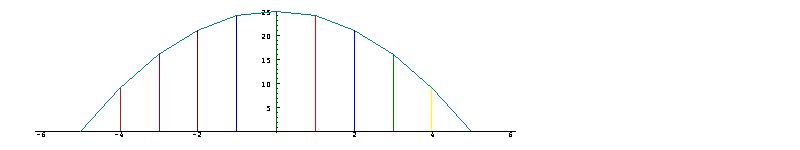 A plot can be removed
from the screen
(to permit further
computation) by
pressing
the key labelled Esc.
However, anyone
unfamiliar with such
graphs should perhaps
make a few by hand,
using simple
functions such as the
cube
(
A plot can be removed
from the screen
(to permit further
computation) by
pressing
the key labelled Esc.
However, anyone
unfamiliar with such
graphs should perhaps
make a few by hand,
using simple
functions such as the
cube
(f=: ^ with 3),
negation
(f=: -),
and
the identity
(f=: ]).
x,:fs x
or
x,.fs x
to make its table,
and compare your
observations with
the
remarks given
below:
fs=: 0 1 0 _1r6 0 1r120 0 _1r5040 with p.
x=: 1r3*i:10
PLOT x;fs x
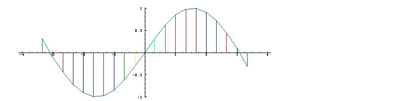
fs
appears to be an
oscillating
function that
begins at about
(-3+1r7),0;
drops at a
decreasing
rate to a low of
_1;
rises
through
0 0
to a high of
1;
and again
drops to about
(3+1r7),0.
PLOT x;f x
is said to be a
plot of
f x
"against" or
"versus" the
argument
x. A
function can also
be plotted
against another
function, as
illustrated
in the following
exercise.
fc=: 1 0 _1r2 0 1r24 0 _1r720 0 1r40320 with p.
set 5
x,.fc x
PLOT x;fc x
(fc x),.(fs x)
PLOT (fc x);(fs x)
fs
and
fc
are
approximations of
them.
fs
against
fc in
the preceding
exercise
produced an
approximate
circle.
d,:e
produces a
two-rowed table
from the
lists
d and
e,
and
expressions of the
form
c,d,:e
form multi-rowed
tables from
further lists.
Moreover,
PLOT x;c,d,:e
plots each of the
lists against
x in
a single graph,
providing visual
comparison of the
functions
represented by the
lists.
PLOT x;(fs x),:fc x)
PLOT x;(fs x),:fc x-3r2)
3B.
Local behaviour
and area
S3B.
cir=: 0 with o.
gives the square
root of one minus
the square
of its argument.
Its plot for the
argument
a=: 1r5*i:5
is therefore a
rough
approximation to a
semi-circle with a
radius of one
unit. Thus:
cir=: 0 with o.
a=: 1r5 * i:5
a
_1 _4r5 _3r5 _2r5 _1r5 0 1r5 2r5 3r5 4r5 1
PLOT a;cir a
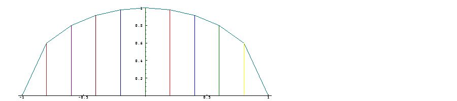
sum=: +/
sums a list, and
sum cir a
therefore sums the
altitudes of the
graph of the
semi-circle, thus
giving an
approximation to
its area
(except that the
sum must be
multiplied
by
1r5,
the common width
of the
trapezoids that
form the area).
Thus:
sum=: +/
1r5 * sum cir a
1.51852
2*1r5 * sum cir a
3.03705
pi.
Better
approximations are
provided by a
larger
number of points:
b=: 1r1000 * i:1000
2 * +/1r1000 * cir b
3.14156
3C.
Graphs versus
function
tables
S3C.
Insights provided by
the graph of the
function
cir that
are not provided so
directly by its
function table are
based upon the
pairwise views of
adjacent points;
the slopes of the
line segments between
them reflect the rate
of change of the
function, and the
trapezoids defined by
them provide a basis
for the area.
pw, a
sum function, a
commuted
difference
function, and an
average or
mean function.
Thus:
pw=: 1 : '2 with (u.\)'
sum=: +/
dif=: -~/
mean=: sum % #
y=: cir a
y
0 0.6 0.8 0.917 0.98 1 0.98 0.917 0.8 0.6 0
mean y
0.69
mean pw y NB. Average heights of the trapezoids
0.3 0.7 0.86 0.95 0.99 0.99 0.95 0.86 0.7 0.3
dif pw y
0.6 0.2 0.12 0.063 0.02 _0.02 _0.063 _0.12 _0.2 _0.6
We will further
illustrate the
pairwise
operator on a
function for the
Fibonacci
numbers, using a
definition discussed
under "generating
functions" in [2]:
fib=: (0 1 with p. % 1 _1 _1 with p.)t.
x=: 1 2 3 4 5 6 7 8 9 10 11 12 13
fib x
1 1 2 3 5 8 13 21 34 55 89 144 233
sum pw fib x
2 3 5 8 13 21 34 55 89 144 233 377
sum pw sum pw fib x
5 8 13 21 34 55 89 144 233 377 610
dif pw fib x
0 1 1 2 3 5 8 13 21 34 55 89
gm=: %/pw fib x NB. Pairwise ratios
set 4
gm NB. Appproximations to golden mean
1 0.5 0.6667 0.6 0.625 0.6154 0.619 0.6176 0.6182 0.618 0.6181 0.618
gm * 1 + gm
2 0.75 1.111 0.96 1.016 0.9941 1.002 0.9991 1 0.9999 1 1
dif pw f x
are
easily seen in a
graph of
f,
but
repeated use (as
in
dif pw dif pw f x)
are
not. They can,
however,
provide
interesting
results when
applied to
familiar
functions. For
example:
sqr=: ^ with 2
sqr x
1 4 9 16 25 36 49 64 81 100 121 144 169
dif pw sqr x
3 5 7 9 11 13 15 17 19 21 23 25
dif pw dif pw sqr x
2 2 2 2 2 2 2 2 2 2 2
dif pw dif pw dif pw sqr x
0 0 0 0 0 0 0 0 0 0
dp=: dif pw
dp sqr x
3 5 7 9 11 13 15 17 19 21 23 25
dp dp sqr x
2 2 2 2 2 2 2 2 2 2 2
cube=: ^ with 3
cube x
1 8 27 64 125 216 343 512 729 1000 1331 1728 2197
dp cube x
7 19 37 61 91 127 169 217 271 331 397 469
dp dp cube x
12 18 24 30 36 42 48 54 60 66 72
dp dp dp cube x
6 6 6 6 6 6 6 6 6 6
p2=: 2 with ^
and the use
of the
pair-wise
quotients
%/ pw
and
%~/ pw
on it.
3D.
Notes
S3D.
Chapters 2 and 3
introduced two
important
facilities for the
study of functions,
the
function table, and
graphs. Chapter 1
introduced one
particularly
important
function, the
polynomial --
important
because it can
approximate, and
therefore be
used to study, a wide
range of functions.
The next chapter
examines it further.
* for
both
signum and
multiplication in
Section 1D) may
wish to turn now
to the two-page
discussion of
trains,
inflections,
ambivalence,
and bonding in
Section 10D.
4A.
Bonding4A.
Bonding
S4A.
The
polynomial
function
introduced
in
Chapter 1
is a
function
of two
arguments,
the first
of which
is
commonly
called
the
coefficients
of the
function.
Using the
example
from
Chapter
1:
x=: 4
2 3 4 p. x
78
c=: 2 3 4
c p. x
78
g=: c with p.
g x
78
The
expression
g=: c with p.
illustrates
the
fact that
the
function
p.
can be
bonded
with a
list of
coefficients
to define
a
specific
polynomial
function
g.
Consider
the
following
examples:
c2=: 1 2 1
c3=: 1 3 3 1
c4=: 1 4 6 4 1
y=: 0 1 2 3 4 5
f2=: c2 with p.
f2 y
1 4 9 16 25 36
f3=: c3 with p.
f3 y
1 8 27 64 125 216
(f2 y) * (f3 y)
1 32 243 1024 3125 7776
g=: f2 * f3
g y
1 32 243 1024 3125 7776
The
Taylor
operator
t.
applies
to a
polynomial
such as
f3
to
produce a
function
which,
applied
in turn
to an
integer
i,
gives
coefficient
i
of the
polynomial.
For
example:
f3 t. 2
3
f3 t. 0 1 2 3 4 5 6
1 3 3 1 0 0 0
(f2 * f3) t. 0 1 2 3 4 5 6
1 5 10 10 5 1 0
The
result of
f2 f3 y
is said
to be the
result
of
applying
f2
to the
result of
f3.
The
corresponding
function
is
denoted
by
f2 on f3.
For
example:
f3 y
1 8 27 64 125 216
f2 1 8 27 64 125 216
4 81 784 4225 15876 47089
f2 f3 y
4 81 784 4225 15876 47089
h=: f2 on f3
h y
4 81 784 4225 15876 47089
h t. 0 1 2 3 4 5 6 7 8
4 12 21 22 15 6 1 0 0
g1=: f2 * f2
g2=: f2 * f2 * f2
g3=: f3 - f2
g4=: f3 on g
SUM c with p. + d with p.
DIFFERENCE c with p. - d with p.
PRODUCT c with p. * d with p.
COMPOSITION (c with p.) on (d with p.)
SLOPE or rate of increase over an interval
DERIVATIVE or limit of the slope over small intervals
AGGREGATE or area under the graph of a function
INTEGRAL or limit of the area for small intervals
4B.
Notes
S4B.
This
brief
treatment
of
polynomials
is enough
to
provide a
basis for
the
treatment
of the
important
topics of
Power
Series,
Slope and
Derivative,
Growth
and
Decay,
and
Vibrations
in the
next four
chapters.
We
therefore
defer
further
discussion
of
the
polynomial
to
Chapter
16:
Polynomials
and
Number
Systems.
That
chapter
may,
however,
be
attempted
at any
point.
5A.
Introduction
5A.
Introduction
S5A.
Elements
of
a
list
may
be
identified
and
selected
by
its
indices,
beginning
at
zero.
For
example:
a=: 1 2 3 4 5 6 ^ 3
a
1 8 27 64 125 216
0 { a
1
1 { a
8
5 { a
216
6 { a
|index error
| 6 {a
A
polynomial
whose
coefficients
may
be
expressed
as
a
function
of
their
indices
is
called
a
power
series.
For
example:
g=: ! with 3
g i. 8
1 3 3 1 0 0 0 0
(g i.8) with p. 0 1 2 3 4 5 6
1 8 27 64 125 216 343
g 0
gives
the
number
of
distinct
ways
that
zero
things
can
be
chosen
from
three
things;
g 1
gives
the
number
of
ways
that
one
thing
can
be
chosen,
and
so
on,
to
the
case
g 4
which
shows
that
four
things
can
be
chosen
from
three
in
no
ways.
The
resulting
coefficients
are
those
used
in
c3
in
Section
4A;
h=: ! with 4
gives
those
used
in
c4,
and
so
on.
The
coefficients:
0 1 0 _1r6 0 1r120 0 _1r5040
1 0 _1r2 0 1r24 0 _1r720 0 1r40320
used
in
Section
3A
can
also
be
expressed
as
power
series.
Both
lists
are
reciprocal
factorials
(such
as
1r24
and
1r120)
multiplied
by
_1
or
0
or
1.
The
power
series
function
for
the
first
is
given
by:
ps=: % on ! * 2 with | * _1: ^ 3: = 4: | ]
ps 0 1 2 3 4 5 6 7 8 9 10r1
0 1 0 _1r6 0 1r120 0 _1r5040 0 1r362880 0
pc
for
the
second
list
of
coefficients
given
above.
5B.
Truncated
power
series
S5B.
For
the
power
series
g=: ! with 3,
the
coefficients
following
the
first
four
are
all
zero,
and
the
truncated
series
g i.4
therefore
defines
a
polynomial
that
is
equivalent
to
the
longer
list
produced
by
g i.8.
Thus:
g i.4
1 3 3 1
(g i.4) with p. x=: 0 1 2 3 4 5 6
1 8 27 64 125 216 343
g i.8
1 3 3 1 0 0 0 0
(g i.8) with p. x
1 8 27 64 125 216 343
ps=: % on ! * 2 with | * _1: ^ 3: = 4: | ]
never
"terminates"
with
all
zeros.
However,
the
reciprocal
factorial
factor
(% on !)
ensures
that
successive
terms
diminish
rapidly
in
magnitude,
and
a
short
series
may
therefore
provide
a
good
approximation.
For
example:
] c12=: ps i. 12r1
0 1 0 _1r6 0 1r120 0 _1r5040 0 1r362880 0 _1r39916800
] c10=: ps i. 10r1
0 1 0 _1r6 0 1r120 0 _1r5040 0 1r362880
set 9
dec (c12 with p. ,c10 with p.) 2
0.909296136 0.909347443
However,
the
definition
of
the
polynomial
in
Section
1I
shows
that
successive
coefficients
are
multiplied
by
successive
powers
of
the
argument
x.
For
large
arguments,
the
growth
of
this
factor
may
be
fast
enough
to
overpower
the
decrease
in
the
coefficient.
For
example:
dec (c12 with p. ,c10 with p.) 5
_1.1336173 0.08963018
For
small
arguments
(particularly
for
those
less
than
one
in
magnitude),
reasonably
short
power
series
of
the
type
that
includes
a
reciprocal
factorial
factor
provide
good
approximations.
For
example:
dec ((ps i.20) with p.,(ps i.18) with p.) 5
_0.958933165 _0.958776369
y=: 1r5 * i:5
y
_1 _4r5 _3r5 _2r5 _1r5 0 1r5 2r5 3r5 4r5 1
sin=: 1 with o.
((ps i.10) with p.,.(ps i.8) with p.,.sin) y
_0.841471010 _0.841468254 _0.841470985
_0.717356093 _0.717355723 _0.717356091
_0.564642473 _0.564642446 _0.564642473
_0.389418342 _0.389418342 _0.389418342
_0.198669331 _0.198669331 _0.198669331
0 0 0
0.198669331 0.198669331 0.198669331
0.389418342 0.389418342 0.389418342
0.564642473 0.564642446 0.564642473
0.717356093 0.717355723 0.717356091
0.841471010 0.841468254 0.841470985
t.
can
be
used
to
produce
the
power
series
for
the
sine
as
follows:
sin t. i. 12r1
0 1 0 _1r6 0 1r120 0 _1r5040 0 1r362880 0 _1r39916800
sign sin t. i. 12r1
0 1 0 _1 0 1 0 _1 0 1 0 _1
^
q=: (^t.i),.(1 with o.t.i),.(2 with o.t.i=: i.12x)
q,.*q
5C.
Notes
S5C.
Power
series
are
of
great
importance
in
math,
and
it
is
tempting
to
digress
in
a
discussion
of
reasons
for
this
importance,
much
as
was
done
for
polynomials
in
Section
4A.
6A.
Approximation
to
the
derivative
(rate
of
change)
6A.
Approximation
to
the
derivative
(rate
of
change)
S6A.
As
remarked
in
Section
3B,
the
slopes
of
the
segments
of
a
graph
show
the
average
rate
of
change
of
a
function
between
adjacent
points.
Plotting
more
points
at
lesser
intervals
gives
a
better
approximation.
For
example:
c=: 4 _3 _2 1
f=: c with p.
x1=: i.4
PLOT x1;f x1
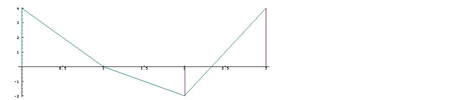 x2=: 1r10*i.31
PLOT x2;f x2
x2=: 1r10*i.31
PLOT x2;f x2
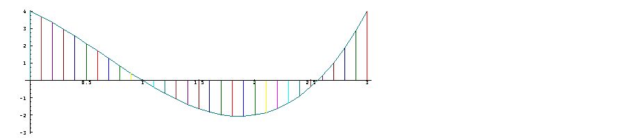 x3=: 1r100 * i.301
PLOT x3;f x3
x3=: 1r100 * i.301
PLOT x3;f x3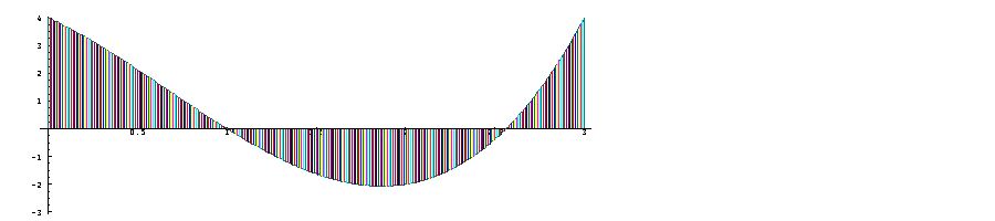
((f x+r)-(f x))%r gives
the
slope
of
the
graph
of
f
between
arguments
x
and
x+r
as
the
ratio
of
the
rise
(f x+r)-(f x)
to
the
run
r.
For
example:
x=: 2
r=: 1r10
((f x+r)-(f x)) % r
1.41
x=: 0 1 2 3 4 5 6
r=: 1r1000
((f x+r)-(f x)) % r
_3.002 _3.999 1.004 12.007 29.01 52.013 81.016
r=: 1r10000
((f x+r)-(f x)) % r
_3.0002 _3.9999 1.0004 12.001 29.001 52.001 81.002
For
these
small
values
of
the
run,
the
slopes
appear
to
be
"approaching
a
limiting
value"
given
approximately
by
the
run
of
one
ten-thousandth.
This
limiting
value
is
the
derivative
of
the
function
f,
that
is,
the
slope
of
the
tangent.
The
value
r=: 0
might
seem
appropriate,
but
this
only
gives
the
meaningless
division
of
a
zero
rise
by
a
zero
run.
Thus:
r=: 0
((f x+r)-(f x)) % r
0 0 0 0 0 0 0
The
desired
result
is
given
by
the
derivative
operator
d.,
with
f d.1
giving
the
(first)
derivative
of
f
and
f d.2
giving
the
second
derivative
(that
is,
the
derivative
of
the
derivative),
and
so
on.
For
example:
f d.1 x
_3 _4 1 12 29 52 81
f d.2 x
_4 2 8 14 20 26 32
f d.1 2 3 4 5 x
_3 _4 6 0 0
_4 2 6 0 0
1 8 6 0 0
12 14 6 0 0
29 20 6 0 0
52 26 6 0 0
81 32 6 0 0
Moreover,
the
application
of
the
Taylor
operator
to
the
resulting
derivatives
show
them
to
be
terminating
power
series,
that
is,
ordinary
polynomials:
d=: f d.1 t. i.7
d
_3 _4 3 0 0 0 0
f d.2 t. i.7
_4 6 0 0 0 0 0
d with p. x
_3 _4 1 12 29 52 81
d with p. d.1 x
_4 2 8 14 20 26 32
f d.2 x
_4 2 8 14 20 26 32
The
coefficients
d
of
the
first
derivative
polynomial
must
bear
some
relation
to
the
coefficients
c
of
the
original
polynomial
f.
We
will
explore
this
relation
by
examining
their
ratios,
as
seen
in
their
divide
table:
d % table c
+--+----------------+
| | 4 _3 _2 1|
+--+----------------+
|_3|_3r4 1 3r2 _3|
|_4| _1 4r3 2 _4|
| 3| 3r4 _1 _3r2 3|
| 0| 0 0 0 0|
| 0| 0 0 0 0|
| 0| 0 0 0 0|
| 0| 0 0 0 0|
+--+----------------+
The
diagonal
of
successive
integers
1 2 3
suggests
that
d
may
be
obtained
from
c
by
multiplying
by
successive
integers,
and
rotating
the
result
one
place
to
the
left:
c
4 _3 _2 1
#c NB. number of elements in c
4
i.#c
0 1 2 3
c * i.#c
0 _3 _4 3
1 |. c * i.#c
_3 _4 3 0
d
_3 _4 3 0 0 0 0
We
will
first
test
this
relation
on
another
polynomial
function
and
then,
in
the
following
section,
examine
the
question
of
why
the
relation
holds
in
general:
c2=: ! with 5 i.6
c2
1 5 10 10 5 1
f2=: c2 with p.
d2=: f2 d.1 t. i.5
d2
5 20 30 20 5
1 |. c2 * i.#c2
5 20 30 20 5 0
6B.
Derivatives
of
polynomials
S6B.
The
polynomial
f=: 4 1 3 2 with p.
is
a
sum
of
four
monomials.
Thus:
f=: 4 1 3 2 with p.
f0=: 4 with * on (^ with 0)
f1=: 1 with * on (^ with 1)
f2=: 3 with * on (^ with 2)
f3=: 2 with * on (^ with 3)
(f0,f1,f2,:f3) x
4 4 4 4 4 4 4
0 1 2 3 4 5 6
0 3 12 27 48 75 108
0 2 16 54 128 250 432
(f0+f1+f2+f3) x
4 10 30 76 160 294 490
f x
4 10 30 76 160 294 490
Any
slope
of
a
function
that
is
a
sum
of
functions
equals
the
sum
of
the
corresponding
slopes
of
the
component
functions,
and
the
derivative
of
a
sum
of
functions
is
therefore
the
sum
of
the
derivatives
of
the
corresponding
functions.
For
example:
(f0 d.1 , f1 d.1 , f2 d.1 ,: f3 d.1) x
0 0 0 0 0 0 0
1 1 1 1 1 1 1
0 6 12 18 24 30 36
0 6 24 54 96 150 216
(f0 d.1 + f1 d.1 + f2 d.1 + f3 d.1) x
1 13 37 73 121 181 253
f d.1 x
1 13 37 73 121 181 253
Similar
remarks
apply
to
the
multiplication
that
occurs
in
the
monomials.
For
example,
in
f2=: 3 with * on (^ with 2),
the
multiplication
by
three
of
the
square
function
(^ with 2)
multiplies
each
of
its
slopes
by
three,
and
therefore
multiplies
its
derivative
by
three.
It
remains
to
determine
the
derivative
of
power
functions
such
as
the
square.
If
f=: ^ with 2,
then
the
rise
(f x+r)-(f x)
is
given
by
the
square
of
x+r
(that
is,
(x+r)*(x+r))
minus
the
square
of
x.
x
plus
2*x*r
plus
the
square
of
r,
and
subtraction
of
the
square
of
x
then
leaves
a
rise
of
2*x*r
plus
the
square
of
r.
The
slope
of
the
square
function
(for
the
run
r)
is
then
given
by
dividing
this
sum
by
r
to
obtain
(2*x)+r.
The
derivative
is
then
given
by
the
case
for
r=: 0,
that
is,
2*x
(or,
equivalently,
2*x^1).
(x+r)*(x+r)*(x+r)gives
3*x^2
for
the
derivative
of
the
cube
^ with 3,
and,
in
general,
gives
n*x^(n-1)for
the
derivative
of
^ with n.
The
contribution
of
a
monomial
cn * x ^ n
to
the
derivative
polynomial
is
therefore
the
monomial
n * cn * x ^ (n-1),
which
therefore
appears
as
a
coefficient
n * cn
displaced
one
place
to
the
left
in
the
list
of
coefficients.
d=: 1: |. c * i.#c
given
in
the
preceding
section
for
the
coefficients
d
of
the
derivative
polynomial.
These
results
will
be
summarized
by
defining
a
function
der
which,
applied
to
a
list
of
coefficients
of
a
polynomial,
gives
the
list
of
coefficients
of
the
derivative
polynomial.
We
will
illustrate
its
use
on
the
polynomial
graphed
in
Section
A,
and
will
graph
it
together
with
the
secant
slopes
of
the
function
so
that
they
can
be
compared:
der=: 1: |. ] * i. on #
c=: 4 _3 _2 1
d=: der c
d
_3 _4 3 0
x2=: 1r10*i.31
PLOT x2 ; (c with p. ,: d with p.) x2
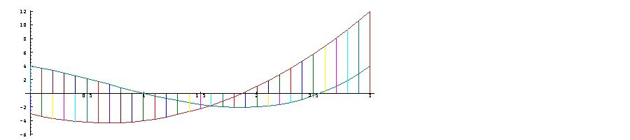
f
correctly
suggests
that
it
is
a
function
derived
from
f,
but
it
is
only
one
among
many
(such
as
the
inverse)
also
derived
from
f.
The
phrase
slope
of
f
would
be
more
informative,
and
could
be
distinguished
from
the
associated
secant
slope
of
f.
6C.
Taylor
coefficients
S6C.
It
is
also
interesting
to
compare
the
Taylor
coefficients
of
the
derivative
of
the
polynomial
d with p.
with
the
result
of
the
function
der:
d with p. d.1 t. i.8
_4 6 0 0 0 0 0 0
der d
_4 6 0 0
As
a
foretaste
of
the
growth
and
oscillating
functions
of
the
next
two
chapters,
we
will
also
show
Taylor
series
for
the
exponential
and
sine
functions:
exp=: ^
exp t. i=: i.10r1
1 1 1r2 1r6 1r24 1r120 1r720 1r5040 1r40320 1r362880
exp d.1 t. i
1 1 1r2 1r6 1r24 1r120 1r720 1r5040 1r40320 1r362880
exp d.2 t. i
1 1 1r2 1r6 1r24 1r120 1r720 1r5040 1r40320 1r362880
sin=: 1 with o.
]s=: sin t. i.12r1
0 1 0 _1r6 0 1r120 0 _1r5040 0 1r362880 0 _1r39916800
der s
1 0 _1r2 0 1r24 0 _1r720 0 1r40320 0 _1r3628800 0
sin d.1 t. i.11r1
1 0 _1r2 0 1r24 0 _1r720 0 1r40320 0 _1r3628800
der der s
0 _1 0 1r6 0 _1r120 0 1r5040 0 _1r362880 0 0
der der der s
_1 0 1r2 0 _1r24 0 1r720 0 _1r40320 0 0 0
der der der der s
0 1 0 _1r6 0 1r120 0 _1r5040 0 0 0 0
s
0 1 0 _1r6 0 1r120 0 _1r5040 0 1r362880 0 _1r39916800
6D.
Notes
S6D.
For
an
arbitrary
function
f
(such
as
any
one
of
the
functions
of
trigonometry),
the
matter
of
the
limiting
value
of
the
secant
slope
((f x+r)-(f x)) % r
as
r
"approaches"
zero
(discussed
in
Section
6A)
raises
difficult
questions
that
are
properly
answered
only
by
lengthy
analysis
of
the
notion
of
limits.
This
is
what
makes
Calculus
such
a
forbidding
subject.
f
is
a
good
approximation
to
the
derivative
of
f
?
Yes,
but
only
for
functions
that
are
"uniformly
continuous".
This
is
true
of
a
wide
range
of
functions
of
practical
interest,
including
all
of
those
to
be
treated
in
subsequent
chapters.
7A.
Growth
polynomials
7A.
Growth
polynomials
S7A.
It
is
a
common
observation
that
growing
things
(such
as
young
plants
and
animals,
young
commercial
companies,
and
a
colony
of
bacteria)
change
not
at
a
constant
rate,
but
at
a
rate
roughly
proportional
to
present
size.
^
.
In
a
graph
of
this
function
this
relation
may
be
seen
approximately
in
the
slopes
of
the
secants.
Thus:
x=: 1r2*i.11
x
0 1r2 1 3r2 2 5r2 3 7r2 4 9r2 5
set 4
^ x
1 1.649 2.718 4.482 7.389 12.18 20.09 33.12 54.6 90.02 148.4
PLOT x;^x
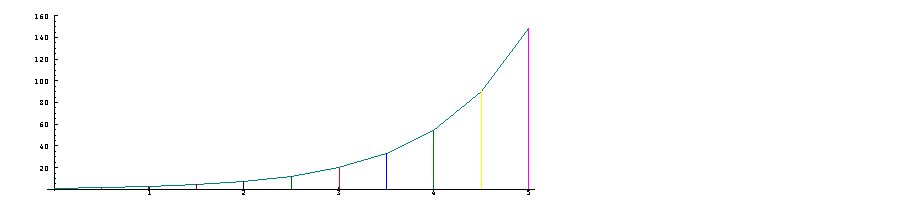
c=: 1 1 1r2 1r6 1r24 1r120 1r720 1r5040
der=: 1:|.]*i.@:# NB. Gives coeffs of derivative
d=: der c
d
1 1 1r2 1r6 1r24 1r120 1r720 0
dec c with p. x
1 1.649 2.718 4.481 7.381 12.13 19.85 32.23 51.81 82.22 128.6
dec d with p. x
1 1.649 2.718 4.478 7.356 12.01 19.41 30.95 48.56 74.81 113.1
The
two
polynomials
differ
only
in
the
term
1r5040*x^7,
and
are
therefore
nearly
equal
for
reasonably
small
values
of
x.
Moreover,
the
pattern
required
of
further
coefficients
is
clear:
coefficient
k
must
be
1%!k.
Thus:
! i. 12r1
1 1 2 6 24 120 720 5040 40320 362880 3628800 39916800
a=: 1 % ! i. 12
b=: der a
(a with p. ,. b with p. ,. ^) x
1 1 1
1.649 1.649 1.649
2.718 2.718 2.718
4.482 4.482 4.482
7.389 7.389 7.389
12.18 12.18 12.18
20.08 20.08 20.09
33.11 33.08 33.12
54.55 54.44 54.6
89.8 89.42 90.02
147.6 146.4 148.4
^(x+3)
and
(^x) * (^3),
and
comment
on
the
results.
(^x) * (^-x)
^(x+-x)
set 2
^-x
% ^ x
decay=: ^ on -
decay x
decay t. i. 10
7B.
The
name
Exponential
S7B.
^,
the
expression
x^e
is
said
to
denote
the
base
x
to
the
exponent
e,
and
the
function
x with ^
may
therefore
be
said
to
be
an
exponential
function.
For
example:
e=: 1r10*i.11
e
0 1r10 1r5 3r10 2r5 1r2 3r5 7r10 4r5 9r10 1
3^e
1 1.1 1.2 1.4 1.6 1.7 1.9 2.2 2.4 2.7 3
3 with ^ e
1 1.1 1.2 1.4 1.6 1.7 1.9 2.2 2.4 2.7 3
^e
1 1.1 1.2 1.3 1.5 1.6 1.8 2 2.2 2.5 2.7
2 with ^ e
1 1.1 1.1 1.2 1.3 1.4 1.5 1.6 1.7 1.9 2
The
exponential
function
^
appears
to
lie
between
the
functions
2 with ^
and
3 with ^.
Thus:
set 7
(^,.2.5 with ^,.2.75 with ^,.2.71 with
^,.2.718 with ^,.1x1 with ^) e
1 1 1 1 1 1
1.105171 1.095958 1.106454 1.104834 1.105159 1.105171
1.221403 1.201124 1.22424 1.220658 1.221377 1.221403
1.349859 1.316382 1.354565 1.348624 1.349817 1.349859
1.491825 1.4427 1.498763 1.490005 1.491763 1.491825
1.648721 1.581139 1.658312 1.646208 1.648636 1.648721
1.822119 1.732862 1.834846 1.818786 1.822005 1.822119
2.013753 1.899144 2.030172 2.009456 2.013607 2.013753
2.225541 2.081383 2.246292 2.220115 2.225356 2.225541
2.459603 2.281109 2.485418 2.452858 2.459374 2.459603
2.718282 2.5 2.75 2.71 2.718 2.718282
The
base
that
gives
the
exponential
exactly
is
called
Euler"s
number,
and
is
denoted
in
math
by
e
and
in
J
by
1x1
.
8A.
Introduction
8A.
Introduction
S8A.
Vibrations
are
commonly
seen
in
the
motions
of
a
clock
pendulum,
of
a
piano
string,
and
of
a
weight
(such
as
a
plumb
bob
suspended
on
a
rubber
band
or
steel
spring).
If
the
bob
is
pulled
straight
down
a
certain
distance
from
its
rest
position
and
released,
it
visibly
oscillates
above
and
below
its
rest
position
until
it
is
brought
to
rest
by
friction
in
the
air
and
in
the
suspension.
b
is
a
function
that
gives
the
position
of
the
bob
as
a
function
of
time,
then
its
speed
or
velocity
is
given
by
b d.1
(the
rate
of
change
of
position),
and
its
acceleration
is
given
by
the
second
derivative
b d.1 d.1
(the
rate
of
change
of
its
velocity).
b
of
the
bob.
In
other
words,
the
second
derivative
b d.1
is
proportional
to
-b.
-b
is
equal
to
b d.1 d.1,
and
we
seek
a
polynomial
with
this
property.
Consider
the
coefficients
of
the
function
fs
introduced
in
Section
3A:
c=: 0 1 0 _1r6 0 1r120 0 _1r5040
der c
1 0 _1r2 0 1r24 0 _1r720 0
der der c
0 _1 0 1r6 0 _1r120 0 0
-der der c
0 1 0 _1r6 0 1r120 0 0
The
required
pattern
is
clear:
it
is
the
same
as
for
the
exponential
of
Chapter
7,
except
that
alternate
coefficients
are
zero,
and
that
the
other
coefficients
alternate
in
sign.
The
function
with
this
property
is
called
the
sine,
commonly
abbreviated
to
sin:
sin=: 1 with o.
sin t. i.12
0 1 0 _1r6 0 1r120 0 _1r5040 0 1r362880 0
_1r39916800
sin t. 20 21 22 23
0 1r51090942171709440000 0 _1r25852016738884976640000
8B.
Harmonics
S8B.
The
function
sin on (2:*])
applies
the
sin
to
the
double
of
its
argument,
and
therefore
produces
a
vibration
(or
oscillation)
of
twice
the
frequency.
It
is
called
an
harmonic
of
the
oscillation
sin.
This
may
be
seen
in
a
combined
plot
of
the
two
functions:
x=: 1r10 * i.65
plot x;(sin x) ,: (sin on (2:*]) x)
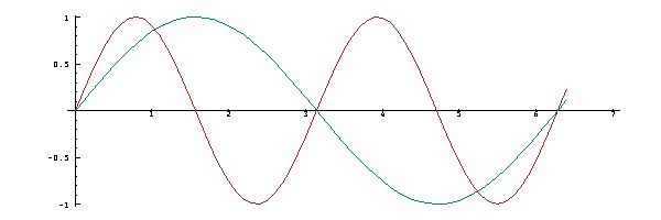
2
in
the
function
sin on (2:*])
by
other
integers
to
produce
other
harmonics,
and
plot
the
results.
cos
and
some
of
its
harmonics.
cos
against
its
harmonic
cos on (2:*]).
8C.
Decay
S8C.
Because
of
"friction"
of
some
sort,
vibrations
commonly
decay,
usually
at
an
approximately
exponential
rate
determined
by
a
function
of
the
form
decay=: ^ on - on (] % [).
sin * 6 with decay .
6,
and
plot
them
together
with
their
non-decaying
counterparts.
9A.
Inverse
9A.
Inverse
S9A.
The
predecessor
function
(<:)
introduced
in
1D
is
said
to
be
the
inverse
of
the
successor
function
(>:)
because
it
"undoes"
its
work.
For
example:
>:1 2 3 4 5
2 3 4 5 6
<:>:1 2 3 4 5
1 2 3 4 5
Conversely,
>:
is
also
the
inverse
of
<:,
and
we
may
simply
say
that
the
two
are
inverses.
h=: (* with 4) on sqr,
where
sqr=: *:
is
the
square
function.
In
order
to
determine
the
voltage
required
to
produce
a
desired
heat,
we
need
the
inverse
v=: sqrt on (% with 4),
where
sqrt=: %:
is
the
square
root
function.
Thus:
h=: (* with 4) on sqr
sqr=: *:
v=: sqrt on (% with 4)
sqrt=: %:
h 0 1 2 3 4 5 6 7
0 4 16 36 64 100 144 196
v h 0 1 2 3 4 5 6 7
0 1 2 3 4 5 6 7
v 0 1 2 3 4 5 6 7
0 0.5 0.707107 0.866025 1 1.11803 1.22474 1.32288
h v 0 1 2 3 4 5 6 7
0 1 2 3 4 5 6 7
For
many
(but
not
all)
functions,
the
inverse
operator
INV=: ^:_1
produces
the
inverse
function.
For
example:
INV=: ^:_1
<:INV 0 1 2 3 4 5 6 7
1 2 3 4 5 6 7 8
cube=: ^ with 3
cuberoot=: cube INV
cube 0 1 2 3 4 5 6 7
0 1 8 27 64 125 216 343
cuberoot cube 0 1 2 3 4 5 6 7
0 1 2 3 4 5 6 7
^ with 4 INV 0 1 2 3 4 5 6 7
0 1 1.18921 1.31607 1.41421 1.49535 1.56508 1.62658
^ with 4 ^ with 4 INV 0 1 2 3 4 5 6 7
0 1 2 3 4 5 6 7
f=: ^ with 3 + ^ with 4
f 0 1 2 3 4 5 6 7
0 2 24 108 320 750 1512 2744
f INV 0 1 2 3 4 5 6 7
|domain error
| f INV 0 1 2 3 4 5 6 7
9B.
Equations
S9B.
However,
for
a
specific
argument,
say
y=: 20,
we
could
find
the
value
of
the
inverse
of
f
by
guessing
the
result
x,
and
applying
f
to
it
to
guide
us
to
an
improved
guess,
by
either
increasing
or
decreasing
x.
For
example:
y=: 20
x=: 2
f x
24
x=: x-1r2
set 5
f x
8.4375
x=: x+1r4
dec f x
14.738
dec f x=: x+1r8
18.951
dec f x=: x+1r16
21.365
dec f x=: x-1r32
20.131
dec f x=: x-1r64
19.535
dec f x=: x+1r128
19.831
dec f x=: x+1r256
19.981
dec f x=: x+1r512
20.056
dec x
1.9043
This
problem
is
commonly
stated
as
the
equation
(f x)=y,
implying
that
one
is
to
find
a
value
of
x
such
that
the
relation
is
true.
Moreover,
the
problem
of
solving
equations
is
commonly
introduced
with
little
or
no
clue
as
to
why
the
matter
is
important.
g=: - with y on f
differs
from
f
in
subtracting
y
from
the
result,
and
a
solution
of
(g x)=0
is
therefore
a
solution
of
(f x)=y.
A
solution
of
(g x)=0
is
said
to
be
a
root
of
the
function
g.
9C.
The
method
of
false
position
S9C.
If
one
knows
two
values
a
and
b
such
that
g a
and
g b
differ
in
sign,
then
a
root
of
g
must
lie
somewhere
between
them;
the
list
ab=: a,b
is
said
to
bracket
the
root.
Evaluation
of
f
at
its
midpoint
m
(that
is,
m=: mean ab)
will
either
yield
zero
(in
which
case
m
is
a
root
of
g),
or
it
will
differ
in
sign
from
one
of
the
two
results
of
g ab.
ab
that
differs
can
be
used
with
m
to
form
a
tighter
bracket,
whose
mean
will
give
a
better
approximation
to
the
root
of
g.
This
process
may
be
repeated
to
obtain
as
close
an
approximation
as
desired.
For
example:
g=: - with y on f
g ab=: 1,2
_18 4
mean=: +/ % #
]m=: mean ab
1.5
g m
_11.563
]ab=: m,1{ab
1.5 2
g ab
_11.563 4
In
general,
a
bracket
of
a
root
of
a
function
g
may
be
tightened
by
the
function
tighten,
defined
and
illustrated
below:
tighten=: mean,(sign on{. on g = sign on g on mean) { ]
tighten ab=: 1,2
1.5 2
tighten tighten tighten ab
1.875 2
g tighten tighten tighten ab
_1.0486 4
The
function
tighten
may
be
paraphrased
as
follows:
Compare
the
sign
of
the
first
element
({.)
of
the
result
of
g
for
equality
with
the
sign
of
g
on
the
mean,
and
use
the
result
(0
or
1)
as
an
index
to
select
from
the
argument;
finally,
catenate
the
selection
with
the
mean.
The
operator
^:
can
be
used
to
apply
a
function
repeatedly,
as
illustrated
below:
tighten^:3 ab
1.875 2
z=: tighten^:0 1 2 3 4 5 6 7 8 9 10 11 12 ab
z;g z
+---------------+-------------------------+
| 1 2| _18 4|
| 1.5 2| _11.5625 4|
| 1.75 2| _5.26172 4|
| 1.875 2| _1.04858 4|
| 1.9375 1.875| 1.36501 _1.04858|
|1.90625 1.875| 0.131333 _1.04858|
|1.89063 1.90625| _0.465246 0.131333|
|1.89844 1.90625| _0.168624 0.131333|
|1.90234 1.90625| _0.0190637 0.131333|
| 1.9043 1.90234| 0.0560301 _0.0190637|
|1.90332 1.90234| 0.018457 _0.0190637|
|1.90283 1.90332|_0.000309859 0.018457|
|1.90308 1.90283| 0.00907195 _0.000309859|
+---------------+-------------------------+
9D.
Newton"s
method
S9D.
If
x=: 2
is
an
appoximation
to
the
root
of
g,
then
(as
suggested
by
the
small
"triangle"
with
apex
at
the
point
x,g x
in
the
accompanying
graph)
a
good
correction
is
provided
by
dividing
g x
by
the
derivative
g d.1 x
that
gives
the
slope
of
the
tangent
to
the
graph
at
the
point
x,g x:
PLOT x;g x=: 1r10*i.22
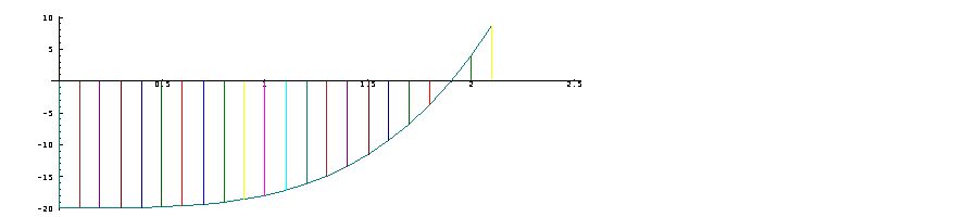
x=: 2
(g , g d.1 , g%g d.1) x
4 44 0.0909091
x=: x - (g%g d.1) x
g x
0.24124
x=: x - (g%g d.1) x
g x
0.00106658
newton=: ] - g % g d.1
newton 2
1.90909
g newton 2
0.24124
newton^:(i.4) 2
2 1.90909 1.90287 1.90284
g newton^:(i.4) 2
4 0.24124 0.00106658 2.1139e_8
g newton ^:(i.3 5) 25
406230 128520 40655 12855.8 4061.08
1279.01 399.129 121.057 33.5929 7.07075
0.658183 0.00775433 1.11692e_6 2.13163e_14 3.55271e_15
g,
its
convergence
is
not
guaranteed
in
general,
especially
for
initial
guesses
far
from
the
root.
9E.
Roots
of
Polynomials
S9E.
The
(possibly
multiple)
roots
of
a
polynomial
c with p.
may,
in
principle,
be
obtained
by
the
methods
of
sections
9C
and
9D,
but
it
may
be
difficult
to
find
suitable
brackets
or
initial
guesses.
However,
the
function
roots=: > on {: on p.
may
be
applied
to
the
coefficients
c
to
obtain
the
roots.
For
example:
roots=: > on {: on p.
c=: _1 0 1
r=: roots c
r
1 _1
c p. r
0 0
d=: 6 1 _4 1
s=: roots d
s
3 2 _1
d p. s
3.55271e_15 2.66454e_15 0
Because
of
the
limited
precision
of
the
computations
leading
to
the
roots
s,
the
application
of
the
polynomial
to
them
yields
tiny
results,
but
not
exact
zeros.
The
following
function
(the
product
of
the
sign
function
with
the
magnitude)
serves
to
make
such
results
more
readable
by
"zeroing"
tiny
results:
zero=: **|
zero d p. s
0 0 0
A
graph
of
the
polynomial
1 0 1 with p.
(one
plus
the
square)
indicates
that
it
has
no
roots,
because
the
graph
never
drops
to
zero:
e=: 1 0 1
x=: i:4
PLOT x;e p. x
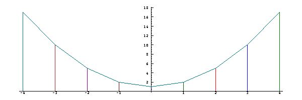
roots
applies
as
follows:
roots e
0j1 0j_1
e p. roots e
0 0
The
root
0j1
is
an
example
of
an
imaginary
number,
to
be
discussed
in
Chapter
19.
Its
square
is
negative
one:
0j1*0j1
_1
9F.
Logarithms
S9F.
The
logarithm
(^.)
is
the
function
inverse
to
the
exponential:
^ ^:_1
^.
^. ^:_1
^
]x=: i.8
0 1 2 3 4 5 6 7
^x
1 2.71828 7.38906 20.0855 54.5982 148.413 403.429 1096.63
^.^x
0 1 2 3 4 5 6 7
^.x
__ 0 0.693147 1.09861 1.38629 1.60944 1.79176 1.94591
^^.x
0 1 2 3 4 5 6 7
As
discussed
in
Section
7B,
the
exponential
^
is
equal
to
e with ^,
where
e=: 1x1
is
Euler's
number.
Similarly,
e with ^.
is
inverse
to
e with ^,
as
illustrated
below:
e=: 1x1
e
2.71828
e with ^ x
1 2.71828 7.38906 20.0855 54.5982 148.413 403.429 1096.63
e with ^. e with ^ x
0 1 2 3 4 5 6 7
10 with ^ x
1 10 100 1000 10000 100000 1e6 1e7
10 with ^. 10 with ^ x
0 1 2 3 4 5 6 7
10 with ^. 1 10 100 1000 10000 100000
0 1 2 3 4 5
The
function
10 with ^.
is
the
base-10
logarithm,
more
commonly
used
in
elementary
math
than
the
natural
log
^.
.
10A.
Introduction
10A.
Introduction
S10A.
Despite
its
importance,
the
grammar
of
our
native
language
is
not
acquired
by
formal
instruction,
but
by
imitation
and
casual
guidance
in
conversation.
Formal
grammar
becomes
important
only
at
a
later
stage,
in
addressing
more
complex
and
more
precise
uses
of
language.
10B.
Word
formation
S10B.
Grammar
is
commonly
taken
to
concern
parsing
the
words
of
a
sentence
into
phrases,
and
determining
the
order
in
which
the
phrases
are
to
be
interpreted.
However,
it
is
worth
noting
that
the
comprehension
of
a
sentence
must
begin
by
first
breaking
it
into
its
component
words.
;: '12+27'
+--+-+--+
|12|+|27|
+--+-+--+
;: '12+.27'
+--+--+--+
|12|+.|27|
+--+--+--+
;: '12+0.27'
+--+-+----+
|12|+|0.27|
+--+-+----+
;: '+/1 2 3 4'
+-+-+-------+
|+|/|1 2 3 4|
+-+-+-------+
The
formal
rules
are
stated
in
the
J
Dictionary
as
follows:
The
alphabet
is
standard
ASCII,
comprising
digits,
letters
(of
the
English
alphabet),
the
underline
(used
in
names
and
numbers),
the
(single)
quote,
and
others
(which
include
the
space)
to
be
referred
to
as
graphics.
It
would
clearly
be
confusing
if
it
were
possible
to
assign
the
name
a.).
e
(as
in
2.4e3
to
signify
2400
in
exponential
form),
and
the
letter
j
to
separate
the
real
and
imaginary
parts
of
a
complex
number,
as
in
3e4j_0.56.
Also
see
the
discussion
of
Constants.
'can''t'
is
the
five-character
abbreviation
of
the
six-character
word
'cannot'.
The
ace
a:
denotes
the
boxed
empty
list
<$0
.
prices=: 4.5 12)
begin
with
a
letter
and
may
continue
with
letters,
underlines,
and
digits.
A
name
that
ends
with
an
underline
or
that
contains
two
consecutive
underlines
is
a
locative,
as
discussed
in
Section
II.I.
+
for
plus)
or
by
a
graphic
modified
by
one
or
more
following
inflections
(a
period
or
colon),
as
in
+.
and
+:
for
or
and
nor.
A
primary
may
also
be
an
inflected
name,
as
in
e.
and
o.
for
membership
and
pi
times.
A
primary
cannot
be
assigned
a
referent.
+
to
multiplication,
as
in
+=: * .
10C.
Parsing
S10C.
The
complete
parsing
rules
are
stated
in
the
J
dictionary
as
follows.
The
leading
five-point
summary
will
suffice
for
most
purposes:
10%3+2,
the
phrase
3+2
is
evaluated
first
to
obtain
a
result
that
is
then
used
to
divide
10.
In
summary:
,"2-a
is
equivalent
to
(,"2)-a,
not
to
,"(2-a).
+/ . */b,
the
rightmost
adverb
/
applies
to
the
verb
derived
from
the
phrase
+/ . *,
not
to
the
verb
* .
3*p%q^|r-5
can
therefore
be
read
from
left
to
right:
the
overall
result
is
3
times
the
result
of
the
remaining
phrase,
which
is
the
quotient
of
p
and
the
part
following
the
%,
and
so
on.
a=: 1 2 3,
then
b=: +/2*a
would
be
parsed
and
executed
as
follows:
" b =: + / 2 * a
" b =: + / 2 * 1 2 3
" b =: + / 2 * 1 2 3
" b =: + / 2 * 1 2 3
" b =: + / 2 * 1 2 3
" b =: + / 2 4 6
" b =: + / 2 4 6
" b =: + / 2 4 6
" b =: 12
" b =: 12
" 12
" 12
The
foregoing
illustrates
two
points:
1)
Execution
of
the
phrase
2 * 1 2 3
is
deferred
until
the
next
element
(the
/)
is
transferred;
had
it
been
a
conjunction,
the
2
would
have
been
its
argument,
and
the
monad
*
would
have
applied
to
1 2 3;
and
2)
Whereas
the
value
of
the
name
a
moves
to
the
stack,
the
name
b
(because
it
precedes
a
copula)
moves
unchanged,
and
the
pronoun
b
is
assigned
the
value
12.
13!:16 (q.v.).
The
executions
in
the
stack
are
confined
to
the
first
four
elements
only,
and
eligibility
for
execution
is
determined
only
by
the
class
of
each
element
(noun,
verb,
etc.,
an
unassigned
name
being
treated
as
a
verb),
as
prescribed
in
the
following
parse
table.
EDGE VERB NOUN ANY 0 Monad
EDGE+AVN VERB VERB NOUN 1 Monad
EDGE+AVN NOUN VERB NOUN 2 Dyad
EDGE+AVN VERB+NOUN ADV ANY 3 Adverb
EDGE+AVN VERB+NOUN CONJ VERB+NOUN 4 Conj
EDGE+AVN VERB VERB VERB 5 Trident
EDGE CAVN CAVN CAVN 6 Trident
EDGE CAVN CAVN ANY 7 Bident
NAME+NOUN ASGN CAVN ANY 8 Is
LPAR CAVN RPAR ANY 9 Paren
Legend: AVN denotes ADV+VERB+NOUN
CAVN denotes CONJ+ADV+VERB+NOUN
EDGE denotes MARK+ASGN+LPAR
10D.
Conventional
mathematical
notation
S10D.
This
section
is
a
discussion
of
mathematical
notation
from
the
vantage
point
of
programming
languages,
with
emphasis
on
ideas
from
programming
that
might
be
adopted
without
conflict
in
mathematical
notation.
By
relieving
the
brain
of
all
unnecesary
work,
a
good
notation
sets
it
free
to
concentrate
on
more
advanced
problems,
and
in
effect
increases
the
mental
power
of
the
race...
By
the
aid
of
symbolism
we
can
make
transitions
in
reasonings
almost
mechanically
by
the
eye...
A.
N.
Whitehead
On
the
other
hand,
Cajori
comments
on
the
paucity
of
publications
concerning
the
general
question
of
notation,
and
quotes
De
Morgan
("a
close
student
of
the
history
of
mathematics")
as
follows:
Mathematical
notation,
like
language,
has
grown
up
without
much
looking
to,
at
the
dictates
of
convenience
and
with
the
sanction
of
the
majority.
In
that
preface
William
Forster
quotes
the
reply
of
Oughtred
to
the
question
of
how
he
(Oughtred)
had
for
so
many
years
concealed
his
invention
of
the
slide
rule
from
himself
(Forster)
whom
he
had
taught
so
many
other
things.
The
reply
was:
On
page
93
Cajori
continues
with:
That
the
true
way
of
Art
is
not
by
Instruments,
but
by
Demonstration:
and
that
it
is
a
preposterous
course
of
vulgar
Teachers,
to
begin
with
Instruments,
and
not
with
the
Sciences,
and
so
in-stead
of
Artists,
to
make
their
Scholers
only
doers
of
tricks,
and
as
it
were
Iuglers
...
That
the
vse
of
instruments
is
indeed
excellent,
if
a
man
be
an
Artist:
but
contemptible
being
set
and
opposed
to
Art.
And
lastly,
that
he
meant
to
commend
to
me,
the
skill
of
Instruments,
but
first
he
would
haue
me
well
instructed
in
the
Sciences.
It
may
be
claimed
that
there
is
a
middle
ground
which
more
nearly
represents
the
ideal
procedure
in
teaching.
Shall
the
slide
rule
be
placed
in
the
student"s
hands
at
the
time
when
he
is
engaged
in
the
mastery
of
principles?
Shall
there
be
an
alternate
study
of
the
theory
of
logarithms
and
of
the
slide
rule
--
on
the
idea
of
one
hand
washing
the
other
--
...
Writing
in
the
early
1900"s,
Cajori
could
not
have
foreseen
the
advent
of
that
universal
mathematical
instrument,
the
modern
computer,
nor
its
spawning
of
the
development
and
study
of
the
notations
of
programming
languages.
00 0080 10
00 0081 11
10 0082 11
loaded
the
number
contained
in
register
80
into
the
accumulator,
added
register
81
to
it,
and
stored
the
resulting
sum
in
register
82.
Let a=3
Let b=5
Let c=(a+b)*(a-b)
Although
a
few
symbols
from
programming
languages
(such
as
FORTRAN"s
*
for
multiplication)
have
been
widely
adopted
in
math,
the
mathematical
notation
used
in
exposition
has
been
largely
unaffected.
On
the
other
hand,
many
mathematicians
have
been
forced
to
learn
programming
languages,
or
to
work
with
programmers
who
translate
their
mathematical
expressions.
"I
doubt
not
but
that
there
shall
be
in
convenient
time,
brought
to
light
many
precepts
which
may
tend
to
ye
perfecting
of
Navigation,
and
the
help
and
safety
of
such
whose
Vocations
doe
inforce
them
to
commit
their
lives
and
estates
in
the
vast
Ocean
to
the
providence
of
God."
Thus
farr
that
very
good
and
judicious
man
Mr.
Oughtred.
I
will
add,
that
if
instead
of
sending
the
Observations
of
Seamen
to
able
Mathematicians
at
Land,
the
Land
would
send
able
Mathematicians
to
Sea,
it
would
signify
much
more
to
the
improvemt
of
Navigation
and
safety
of
Mens
lives
and
estates
on
that
element.
The
need
to
make
translation
manageable
has
led
to
the
development
of
languages
with
simple
and
precisely
defined
grammars,
that
is,
rules
for
word-formation
and
parsing.
Although
mathematical
notation
undoubtedly
possesses
parsing
rules,
they
are
rather
loose,
sometimes
contradictory,
and
seldom
clearly
stated.
It
is
perhaps
significant
that
Cajori"s
History
makes
no
mention
of
the
matter
of
grammar.
v<-2 7 1 8 2 8
+/v
28
The
operator
applies
to
any
function,
such
as
*
(times),
>.
(max),
or
<.
(min),
and
may
therefore
obviate
the
use
of
many
symbols
such
as
the
capital
Greek
sigma
and
pi
for
summation
and
product:
(*/v),(>./v),(<./v)
1792 8 1
Because
of
their
application
to
a
broad
range
of
topics,
their
strict
grammar,
and
their
strict
interpretation,
programming
languages
can
provide
new
insights
into
mathematical
notation.
We
begin
with
the
matter
of
symbols.
= < > _ + * - % ^ $ ~ | . : , ;
# ! / \ [ ] { } " ' ` @ & ?
This
economy
is
achieved
in
part
by
adopting
from
mathematics
the
use
of
reserved
words
such
as
sin,
cos,
e,
and
log
--
reserved
from
use
as
names
for
variables.
Further
economies
are
implicit
in
notions
that
have
been
used
in
mathematics
but
not
systematically
exploited.
We
will
illustrate
them
by
their
use
in
J,
a
language
derived
from
APL.
f
and
g
by
f+g.
This
notion
can
be
exploited
more
generally,
including
constructs
such
as
f+g*h
for
f
added
to
the
product
of
g
and
h.
For
example,
using
%
for
divide,
and
#
for
number
of
elements:
mean=: +/ % # NB. Arithmetic mean or average
mean 1 2 3 4 5
3
com=: ] - +/ % # NB. ] is the identity function
com 1 2 3 4 5 NB. Center on mean
_2 _1 0 1 2
Non-mathematical
functions
can
be
used
in
a
train.
For
example,
the
function
;
(which
boxes
each
argument
and
catenates
the
boxed
results)
can
be
used
to
display
results
for
convenient
comparison:
(];mean;com;] - +/ % #) 1 2 3 4 5
+---------+-+-----------+-----------+
|1 2 3 4 5|3|_2 _1 0 1 2|_2 _1 0 1 2|
+---------+-+-----------+-----------+
1
and
0
to
denote
true
and
false,
and
used
the
symbols
for
times
and
plus
to
denote
the
logical
functions
and
and
or.
*.
for
and
and
+.
for
or.
Similarly,
=
is
used
as
a
truth-function
(like
<
and
>),
whereas
=:
is
used
as
a
copula
(to
assign
a
referent
to
a
name),
and
<.
is
used
for
lesser-of
(that
is,
minimum).
Thus:
p=: 0 0 1 1 [ q=: 0 1 0 1
(p *. q);(p +. q);(p + q);(p < q);(p <. q)
+-------+-------+-------+-------+-------+
|0 0 0 1|0 1 1 1|0 1 1 2|0 1 0 0|0 0 0 1|
+-------+-------+-------+-------+-------+
AMBIVALENCE
In
the
expression
a-b
the
symbol
-
denotes
subtraction
(a
function
of
two
arguments),
whereas
in
-b
it
denotes
negation,
a
different
(albeit
related)
function
of
one
argument.
This
ambivalence
(a
"binding
power"
of
either
two
or
one)
introduces
no
confusion
in
conventional
notation,
and
could
be
exploited
for
other
functions:
a=: 2
b=: 5
(a-b),(-b) NB. Subtraction and Negation (0-b)
_3 _5
(a%b),(%b) NB. Division and Reciprocal (1%b)
0.4 0.2
(a^b),(^b) NB. Power and Exponential (e^b)
32 148.413
(a^.b),(^.b) NB. Base-a log, Natural log (e^.b)
2.32193 1.60944
BONDS
In
their
Combinatory
Logic
[11],
Curry
and
Feys
developed
a
set
of
combinators,
which
we
will
treat
as
operators
in
the
sense
of
Heaviside.
One
of
these
bonds
a
function
of
two
arguments
(such
as
^)
to
one
of
its
arguments
(such
as
3)
to
produce
a
function
of
one
argument
(the
cube),
an
operation
that
has
come
to
be
called
Currying
in
honour
of
its
author.
For
example:
cube=: ^ with 3
log10=: 10 with ^.
(cube ; log10) 10 50 100 200
+-------------------+-------------------+
|1000 125000 1e6 8e6|1 1.69897 2 2.30103|
+-------------------+-------------------+
Conclusion.
Taken
together,
trains,
inflection,
ambivalence,
and
bonds
provide
highly
mnemonic
representations
for
a
host
of
functions.
Their
advantages
can
be
fully
appreciated
only
by
careful
comparison
with
the
alternatives
now
used
in
mathematics.
"727
Invention
of
Symbols.
--
Whenever
the
source
is
known,
it
is
found
to
have
been
individualistic
--
the
conscious
suggestion
of
one
mind.
Comments
about
the
hope
of
grateful
remembrance
appear
unkind;
perhaps
Oughtred
invented
symbols
to
clarify
his
own
thinking,
and
as
a
tool
for
teaching.
Nevertheless,
Cajori"s
main
point
is
sound
--
any
attempt
to
impose
an
individual
system
is
vain
and
hopeless.
log(a+b)*(a-b)
is
carried
out
by
identifying
the
primitive
operations
(such
as
addition)
and
then
performing
them
in
an
appropriate
order.
The
process
begins
with
word-formation
(identification
of
the
individual
words:
log,
left
parenthesis,
a,
+,
b,
etc.),
and
continues
with
parsing
the
sequence
of
words
according
to
a
formal
or
informal
grammar
based
upon
the
parts
of
speech
(variables,
functions,
punctuation,
etc.).
;:)
to
a
quoted
character
string:
;:'log(a+b)*(a-b)'
+---+-+-+-+-+-+-+-+-+-+-+-+
|log|(|a|+|b|)|*|(|a|-|b|)|
+---+-+-+-+-+-+-+-+-+-+-+-+
sqr=: ^ with 2
area=: sqr 4
+/\4#3
3 6 9 12
PARTS OF SPEECH
MATH TERMS ENGLISH (J) TERMS
Constants 2 3 4 Nouns
Variable area Pronoun
Functions ^ # Verbs
Function sqr Proverb
Operators / \ Adverbs
Operator with Conjunction
( ) Punctuation
=: Copula
2+2
and
2*2
and
2^2
yield
identical
results,
only
for
the
specific
argument
2,
but
2*2
and
sqr 2
are
identical
for
any
argument.
Such
an
identity
is
usually
expressed
by
using
a
variable
argument
in
the
form
x*x
and
sqr x
.
pi
in
the
expression
pi=: 3.14159
is
jarring,
since
there
is
no
intent
to
allow
its
value
to
vary.
Although
the
term
pronoun
is
not
commonly
used
in
mathematics,
Hogben
uses
it
(p
432)
to
refer
to
the
symbol
e
used
for
Euler"s
number.
+/v
can
replace
the
Greek
sigma
for
summation
and,
more
generally,
f/
can
replace
other
such
symbols,
but
only
for
functions
that
are
not
anonymous.
x=: 3 [ y=: 4
(x*y),(3*4),(xy),(34) NB. xy is NOT a J expression
12 12 12 34
HIERARCHY
AND
ORDER
OF
EXECUTION
The
polynomial
expression
3x+4x2+2x4
evaluates
correctly
only
under
the
convention
that
the
power
function
is
executed
before
multiplication,
and
multiplication
before
addition.
This
heirarchy
is
adopted
throughout
mathematics,
and
in
almost
all
programming
languages.
+/3 4 2*x^1 2 4,
and
in
+/c*x^e.
1-2-3-4-5
may
be
interpreted
differently
according
to
how
it
is
parenthesized:
the
following
interpretations
are
used
in
mathematics
and
in
J:
(((1-2)-3)-4)-5 NB. Math
1-(2-(3-(4-5))) NB. J
1-(2+3+4+5)),
and
the
J
result
is
the
alternating
sum
(1+3+5)-(2+4).
f/v
inserts
the
function
f
between
elements
of
v,
the
J
expression
-/v
gives
the
alternating
sum,
a
commonly-needed
result
that
is
expressed
in
math
as
the
sum
over
(Greek
sigma)
(-1)i v.
Similarly,
the
alternating
product
is
expressed
as
%/v.
3e6
to
denote
3*10^6.
Producing
no
conflict,
this
has
also
been
widely
adopted
in
mathematics.
3j4
(a
complex
number)
and
1r2
(a
rational)
and
1r2p1
could
be
similarly
adopted
for
many
convenient
constants,
as
illustrated
by
the
following
examples
from
J:
2p1 1r2p1 1r4p_1 NB. Multiples of powers of pi
6.28319 1.5708 0.0795775
3x2 2b101 NB. 3 times e sqared,101 in base 2
22.1672 5
2ad30 NB. Complex number, magnitude 2 at 30 deg.
1.73205j1
n
(when
it
exists)
such
that
n f x
yields
x
for
any
argument
x.
For
example,
0
is
the
neutral
of
+,
and
1
is
the
neutral
of
* .
k{.v
and
k}.v
to
take
and
drop
the
first
k
elements
of
a
vector
v,
we
may
write
identities
concerning
sums
and
products
over
partitions
of
a
vector:
v=: 2 3 5 7 11
k=: 3
(k{.v);(k}.v);((+/k{.v) + (+/k}.v));(+/v)
+-----+----+--+--+
|2 3 5|7 11|28|28|
+-----+----+--+--+
(*/v);((*/k{.v) * (*/k}.v))
+----+----+
|2310|2310|
+----+----+
k=: 0
(for
which
k{.v
is
an
empty
vector),
but
only
because
the
results
of
+/i.0
and
*/i.0
are
defined
to
be
the
neutrals
of
+
and
*.
The
neutral
of
minimum
(<./i.0)
is
infinity,
in
effect
defining
it.
*/x-i.m,
correctly
including
the
case
of
the
empty
vector
that
occurs
when
m
is
zero.
Moreover,
*/x+s*i.m
covers
a
host
of
cases;
in
particular,
the
values
_1
and
0
and
1
for
s
give
the
falling
factorial,
the
ordinary
power
function,
and
the
rising
factorial.
Non-integer
values
of
s
are
equally
useful
in
the
finite
calculus.
!.
provides
them
in
expressions
of
the
form
^!.s.
p.!.s
provides
the
corresponding
polynomial
functions
(in
which
the
power
function
^
used
in
the
ordinary
polynomial
is
replaced
by
the
stope
function
^!.s).
Compare
the
use
of
^!.s
with
the
notations
discussed
in
the
introductory
Note
on
Notation
in
[2].
t under p,
using
the
"under"
operator
under=: &.
.
Thus:
under=: &.
0 0 1 1 +. under -. 0 1 0 1 NB. Or under not is and
0 0 0 1
3 + under ^. 4 NB. Times as add under natural log
12
3 " under (10 with ^.) 4 NB. Division using base-10 log
0.75
(<2 1 3) + under p. (<1 0 4) NB. Add polynomials
+-+------------------+
|2|3.68614 1 0.813859|
+-+------------------+
p.
to
map
the
polynomial
roots
given
by
the
arguments
to
corresponding
coefficients,
which
are
then
added
and
mapped
back
to
give
the
equivalent
multiplier
2
and
roots
3.68614 1 0.813859.
--------------------------------
O O
--------------------------------
O O O
--------------------------------
O
--------------------------------
--------------------------------
Hold the doll
Drop the ball
Drop the ball and hold the doll
I dropped the ball and holded the doll
(base 10) logarithm of 3 log10 3
negation of 3 -3
factorial 3 3! (Order of noun and verb reversed)
(# of combs of) 3 above 5 in large parentheses
3 to the power 5 3 superscript 5
3 beside 5 (3,5) (Parens mandatory for vectors)
this is 3 Let t=3 (Single-letter names only)
that is 5 Let u=5
this plus that t+u
(is) this lessthan that t<u Usually treated as assertions,
(is) this equalto that t=u rather than as more usable truth-
functions that return results
English Math J C
logarithm of 3 log10 3 10^.3 log10(3.0)
negation of 3 3 -3 -3
factorial 3 3! !3 fact(3)
(# of combs of) 3 above 5 in parens 3!5 outof(3,5)
3 to the power 5 3 superscript 5 3^5 pow(3.0,5.0)
3 beside 5 (3,5) 3,5
this is 3 Let t=3 this=: 3 this=3
that is 5 Let u=5 that=: 5 that=5
this plus that t+u this+that this+that
(is) this equalto that t=u this=that this==that
+ - * ^ ! +. *. ^. < = > >:
select
a
few
for
exploration
by
entering
expressions
such
as:
16 + 36
52
16 +. 36
4
x=: 0 1 2 3 4 5
and
y=: x
and
x +/ y
to
produce
an
addition
table.
Then
enter
expressions
for
further
tables
to
identify
each
of
the
functions
listed
in
Exp
1.
Which
of
the
functions
appear
to
be
commutative?
f=: +/*-/
and
g=: </+.=/
]y=: x=: 0 1 2 3 4 5 6 - 3
_3 _2 _1 0 1 2 3
Exp
5
Evaluate
the
familiar
sum
over
(denoted
by
capital
Greek
sigma)
cixi
at
x=0,
assuming
that
(as
is
often
stated)
zero
to
the
power
zero
is
undefined.
2 3 5 7;11 13
x (-/ ; -~/) y
x (</ ; =/ ; g ; <:/) y
~
,
and
state
what
part
of
speech
it
is
in
J:
x (-/ ; -~/) y
x (!/ ; !~/) y
x (*./ ; *.~/) y
S1=: %.S2=: |: (^/%.^!._1/)~ i.10r1
(%. N is matrix inverse, and M %. N is "matrix divide")
;: 'TABLE=: x (*./ ; *.~/) y'
trace=: 13 !: 16
and
9 trace 1
to
invoke
the
tracing
of
subsequent
expressions,
that
is,
to
show
their
detailed
parsing
and
execution.
Then
enter
TABLE=: x (*./ ; *.~/) y
and
other
expressions
from
earlier
explorations.
9 trace 0
.
11A.
Introduction
11A.
Introduction
S11A.
Its
modest
aim
is
to
elaborate
the
point
that
informal,
quasi-empirical,
mathematics
does
not
grow
through
a
monotonous
increase
of
the
number
of
indubitably
established
theorems
but
through
the
incessant
improvement
of
guesses
[Italics
added]
by
speculation
and
criticism,
by
the
logic
of
proofs
and
refutations.
Just
send
me
the
theorems,
then
I
shall
find
the
proofs.
Chrysippus
There
are
then
two
mathematics.
There
is
the
real
mathematics
of
the
real
mathematicians,
and
there
is
what
I
will
call
"trivial"
mathematics,
for
want
of
a
better
word.
The
trivial
mathematics
may
be
justified
by
arguments
which
would
appeal
to
Hogben,
or
other
writers
of
his
school,
but
there
is
no
such
defence
for
the
real
mathematics,
which
must
be
justified
as
an
art
if
it
can
be
justified
at
all.
There
is
nothing
in
the
least
paradoxical
or
unusual
in
this
view,
which
is
that
held
commonly
by
mathematicians.
11B.
Informal
proofs
S11B.
We
will
illustrate
a
proof
by
first
guessing
at
a
relation,
using
the
function
odd
from
Section
2E:
odd=: 1:+2:*i.
odd 6
1 3 5 7 9 11
+/odd 6
36
(+/ odd 1),(+/odd 2),(+/odd 3),(+/odd 4),(+/odd 5)
1 4 9 16 25
It
appears
that
the
sum
of
the
first
n
odd
integers
is
n*n,
a
relation
we
will
demonstrate
by
using
a
few
facts
illustrated
by
the
following:
|. odd 6
11 9 7 5 3 1
(+/odd 6),(+/|.odd 6)
36 36
(odd 6)+(|.odd 6)
12 12 12 12 12 12
6 # 2*6 NB. Six copies of twice six
12 12 12 12 12 12
half=: % with 2
half 6 # 2*6
6 6 6 6 6 6
+/half 6 # 2*6
36
+/6#6
36
6*6
36
We
now
write
a
sequence
of
(obviously?)
equivalent
sentences:
n=: 6
+/odd n
36
+/|.odd n
36
half (+/odd n)+(+/|.odd n)
36
half +/(odd n)+(|.odd n)
36
half +/6 # 2*6
36
+/6 # 6
36
n*n
36
Because
a
value
(6)
was
assigned
to
the
argument
n,
each
of
the
foregoing
sentences
were
executable,
and
were
executed
to
give
results
whose
equality
provided
some
assurance
that
an
error
had
not
been
made.
We
will,
however,
write
an
informal
proof
as
a
similar
sequence,
omitting
the
results
that
would
have
been
produced
by
their
execution.
Thus:
+/odd n
+/|.odd n
half (+/odd n)+(+/|.odd n)
half +/(odd n)+(|.odd n)
half +/6 # 2*6
+/6 # 6
n*n
11C.
Formal
proofs
S11C.
In
a
formal
proof
it
is
necessary
to
state
clearly
the
justification
for
each
equivalence,
that
is,
the
reason
why
each
statement
is
believed
to
be
equivalent
to
the
one
that
precedes
it.
For
example,
we
will
begin
to
convert
the
foregoing
informal
proof
to
a
formal
proof
as
follows:
+/odd n
+/|.odd n
half (+/odd n)+(+/|.odd n)
half +/(odd n)+(|.odd n)
half +/6 # 2*6
+/6 # 6 NB. Half of sum is sum of halves
n*n NB. Def of multiplication (in 1G)
A
stickler
for
logic
might
ask
why
he
should
believe
that
half
of
a
sum
equals
the
sum
of
the
halves
of
the
list
summed.
A
convincing
answer
is
not
as
easy
as
might
be
supposed,
leading
to
an
appreciation
of
the
following
statement
from
Lakatos:
TEACHER:
This
decomposition
of
the
conjecture
suggested
by
the
proof
opens
new
vistas
for
testing.
The
decomposition
deploys
the
conjecture
on
a
wider
front,
so
that
our
criticism
has
more
targets.
+/odd n
and
+/|.odd n?
It
may
seem
obvious,
but
what
is
special
about
+/
that
would
not
apply
for
another
function
such
as
%/
?
A
mathematician
might
say
(and
offer
proofs
that)
functions
such
as
+/
and
*/
and
gcd/
and
>./
are
symmetric,
meaning
that
they
give
the
same
result
when
applied
to
any
permutation
(re-ordering)
of
their
arguments.
TEACHER:
I
agree
with
you
that
the
conjecture
has
received
a
severe
criticism
by
Alpha"s
counterexample.
But
it
is
untrue
that
the
proof
has
"completely
misfired".
If,
for
the
time
being,
you
agree
to
my
earlier
proposal
to
use
the
word
"proof"
for
a
"thought
experiment"
which
leads
to
a
decomposition
of
the
original
conjecture
into
"subconjectures",
instead
of
using
it
in
the
sense
of
a
"guarantee
of
certain
truth",
you
need
not
draw
this
conclusion.
+/even n,
and
write
an
informal
proof
of
the
equivalence.
+/i.n
+/
on i. t. i. 4
11D.
Inductive
proofs
S11D.
+/ on odd n
were
equal
to
n*n
for
a
certain
value
of
n,
we
were
able
to
use
this
assumption
to
prove
that
+/ on odd n+1
must
therefore
equal
(n+1)*(n+1),
we
could
then
conclude
that
equality
must
hold
for
all
succeeding
values,
n+2
and
n+3,
and
so
on.
n=: 0),
we
may
further
conclude
that
the
relation
is
true
for
all
integers
greater
than
or
equal
to
that
value.
For
example:
+/ on odd n+1
(+/odd n)+(2*n)+1 NB. From definition of odd
(n*n)+(2*n)+1 NB. Assumed "induction hypothesis"
(n+1)*(n+1) NB. Simple algebra
11E.
Recursive
definition
S11E.
A
function
that
is
defined
in
terms
of
itself
is
said
to
be
recursively
defined.
For
example,
a
factorial
function
fac
might
be
defined
by
saying
that
fac n
is
n * fac n-1.
However,
it
is
necessary
to
further
define
its
value
for
some
specific
argument;
for
example,
to
define
fac 0
as
1.
]*fac on <:
to
perform
the
recursion,
the
constant
function
1:
for
the
specific
argument
0,
and
the
"conditional
function"
= with 0
to
choose
between
them.
Thus:
fac=: (]*fac on <:) ` 1: @. (= with 0)
fac 0
1
fac 4
24
!4
24
In
the
foregoing,
the
tie
operator
`
forms
a
gerund
from
the
two
functions
to
which
it
is
applied,
and
the
agenda
operator
@.selects
one
of
them
according
to
the
result
of
the
conditional
function
= with 0.
sodd
for
the
sum
of
the
odd
integers
might
be
recursively
defined
as
follows:
sodd=: (sodd on <: + 2 with * - 1:)`0: @. (= with 0)
(sodd 0),(sodd 1),(sodd 2),(sodd 3),(sodd 4)
0 1 4 9 16
The
first
and
"main"
function
of
the
three
used
in
this
recursive
definition
may
be
interpreted
as
follows:
sodd n
is
equal
to
(sodd n-1) + (2*n) " 1
or,
equivalently,
that
sodd n+1
equals
(sodd n) + (2*n+1) " 1.
n
odd
numbers
is
n*n,
using
the
inductive
hypothesis
of
Section
D
as
follows:
sodd n+1
(sodd n) + (2*n+1) " 1 NB. Recursive def of sodd
(n*n) + (2*n+1) " 1 NB. Induction hypothesis
(n+1)*(n+1) NB. Simple algebra
n=: 6
d=: 0 1r6 _1r2 1r3
+/*:i.n
55
d p. n
55
11F.
Guessing
games
S11F.
i.
applies
to
an
argument
such
as
3 4
to
produce
a
table,
but
we
may
also
wish
to
apply
it
to
each
of
the
arguments
3
and
4
to
produce
separate
lists.
Thus:
a=: 3 4
i. a
0 1 2 3
4 5 6 7
8 9 10 11
i.3
0 1 2
i.4
0 1 2 3
eachbox=: &.>
i. eachbox a
+-----+-------+
|0 1 2|0 1 2 3|
+-----+-------+
PREFIX
In
summing
the
list
2 7 1 8,
we
may
also
wish
to
obtain
the
"subtotals"
or
"partial
sums"
by
applying
sumation
over
each
prefix
of
the
list.
Thus:
pref=: \
sum=: +/
a=: 2 7 1 8
sum a
18
sum pref a
2 9 10 18
*/pref a
2 14 14 112
<./pref a
2 2 1 1
>./pref a
2 7 7 8
diag=: /.
c=: 1 2 1
d=: 1 3 3 1
t=: c */d
t
1 3 3 1
2 6 6 2
1 3 3 1
sum diag t
1 5 10 10 5 1
f
is
a
function
and
g
is
a
guess
at
an
equivalent
function,
then
f-g
gives
the
needed
correction.
For
example:
x=: 0 1 2 3 4 5 6 7r1
each=:"0
f=: +/ on i. each NB. Sums of integers
f x
0 0 1 3 6 10 15 21
g=: (^ with 2 % 2:) each
g x
0 1r2 2 9r2 8 25r2 18 49r2
(f-g) x
0 _1r2 _1 _3r2 _2 _5r2 _3 _7r2
corr=: (- % 2:) each
corr x
0 _1r2 _1 _3r2 _2 _5r2 _3 _7r2
gc=: g+corr NB. Corrected guess
(f=gc) x
1 1 1 1 1 1 1 1
RATIOS
The
ratio
f%g
may
sometimes
provide
a
better
guide
to
correction.
Consider,
for
example,
the
following
sums
of
powers:
f1=: +/ on (^&1) on i. each
f2=: +/ on (^&2) on i. each
f3=: +/ on (^&3) on i. each
f4=: +/ on (^&4) on i. each
f5=: +/ on (^&5) on i. each
(f1,f2,f3,f4,:f5) x
0 0 1 3 6 10 15 21
0 0 1 5 14 30 55 91
0 0 1 9 36 100 225 441
0 0 1 17 98 354 979 2275
0 0 1 33 276 1300 4425 12201
For
f1
the
equivalent
function
g1
is,
of
course,
the
function
gc
derived
above,
and
we
will
use
the
ratio
f3%g1
to
look
for
a
definition
of
a
function
g3
corresponding
to
f3.
Thus:
g1=: gc
(f3%g1) x
0 0 1 3 6 10 15 21
g1 x
0 0 1 3 6 10 15 21
It
therefore
appears
that
g3
may
be
expressed
as
the
product
of
g1
with
itself:
g3=: g1*g1
(f3=g3) x
1 1 1 1 1 1 1 1
TAYLOR
COEFFICIENTS
For
functions
such
as
g1
and
g3
that
are
expressed
directly
in
terms
of
powers,
quotients,
products,
and
sums,
the
Taylor
operator
may
be
applied
to
give
the
coefficients
of
an
equivalent
polynomial.
For
example:
x=: 0 1 2 3 4 5 6 7r1
c1=: g1 t. x
c1
0 _1r2 1r2 0 0 0 0 0
c1&p. x
0 0 1 3 6 10 15 21
f1 x
0 0 1 3 6 10 15 21
c3=: g3 t. x
c3
0 0 1r4 _1r2 1r4 0 0 0
(f3=c3&p.) x
1 1 1 1 1 1 1 1
POLYNOMIAL
APPROXIMATIONS
The
Taylor
operator
does
not
apply
to
functions
such
as
the
square
root,
and
we
use
instead
an
expression
that
gives
coefficients
that
approximate
the
function.
Thus:
f=: %:
f x
0 1 1.4142 1.7321 2 2.2361 2.4495 2.6458
(f x)*(f x) NB. To verify that f is square root
0 1 2 3 4 5 6 7
c=: (f x) %. (x ^/ i.#x)
c p. x
0 1 1.4142 1.7321 2 2.2361 2.4495 2.6458
It
may
be
noted
that
the
polynomial
appeared
to
give
not
just
an
approximation,
but
the
exact
result.
However,
the
result
may
be
far
from
correct
for
arguments
other
than
the
x
used
in
computing
the
coefficients,
especially
so
for
arguments
outside
the
range
of
the
elements
of
x.
For
example:
c p. x+1r2
0.64666 1.2301 1.5796 1.8717 2.1204 2.3468 2.5436 2.8157
f x+1r2
0.70711 1.2247 1.5811 1.8708 2.1213 2.3452 2.5495 2.7386
c p. 9
5.9577
f 9
3
12A.
Anagrams
12A.
Anagrams
S12A.
Although
we
have
discussed
the
importance
of
relations
and
analysis
(proofs)
in
math,
our
exclusive
use
of
numeric
arguments
has
probably
given
the
impression
that
math
is
exclusively
about
numbers.
To
redress
the
balance,
we
will
now
treat
some
relations
concerning
English
words,
beginning
with
sorting
and
anagrams.
sort=: /:~ (which applies equally to numeric arguments).
For
example:
sort=: /:~
w0=: 'REVEL'
sort w0
EELRV
w1=: 'LEVER'
sort w1
EELRV
w0=w1
0 1 1 1 0
(sort w0)=(sort w1)
1 1 1 1 1
As
shown
in
the
last
results
the
words
are
not
equal,
but
they
are
similar,
in
the
sense
that
they
are
anagrams,
or
permutations
of
one
another,
containing
the
same
letters
but
in
a
different
order.
Although
it
is
not
an
English
word,
we
will
also
call
the
word
'EELVR'
an
anagram.
w2=: 'AH'
(including
itself).
w3=: 'ART'
.
w4a=: 'SPOT'
.
w4b=: 'ABCD'
.
To
check
your
work,
use
the
anagram
function
A.
as
illustrated
below:
0 A. w2=: 'AH'
AH
1 A. w2
HA
0 1 A. w2
AH
HA
0 1 2 3 4 5 A. w3=: 'ART'
ART
ATR
RAT
RTA
TAR
TRA
6 A. w3
|index error
| 6 A.w3
i.6.
Similar
tests
will
show
that
there
are
twenty-four
anagrams
of
four-letter
words,
leading
to
the
following
tables:
(i.24) A. w4a=: 'SPOT'
SPOT
SPTO
SOPT
SOTP
STPO
STOP
PSOT
PSTO
POST
POTS
PTSO
PTOS
OSPT
OSTP
OPST
OPTS
OTSP
OTPS
TSPO
TSOP
TPSO
TPOS
TOSP
TOPS
trans=: |: NB. Function to transpose a table
trans (i.24) A. w4a=: 'SPOT'
SSSSSSPPPPPPOOOOOOTTTTTT
PPOOTTSSOOTTSSPPTTSSPPOO
OTPTPOOTSTSOPTSTSPPOSOSP
TOTPOPTOTSOSTPTSPSOPOSPS
trans (i.24) A. w4b=: 'ABCD'
AAAAAABBBBBBCCCCCCDDDDDD
BBCCDDAACCDDAABBDDAABBCC
CDBDBCCDADACBDADABBCACAB
DCDBCBDCDACADBDABACBCABA
trans (i.24) A. i.4
0 0 0 0 0 0 1 1 1 1 1 1 2 2 2 2 2 2 3 3 3 3 3 3
1 1 2 2 3 3 0 0 2 2 3 3 0 0 1 1 3 3 0 0 1 1 2 2
2 3 1 3 1 2 2 3 0 3 0 2 1 3 0 3 0 1 1 2 0 2 0 1
3 2 3 1 2 1 3 2 3 0 2 0 3 1 3 0 1 0 2 1 2 0 1 0
(trans (i.24) A. i.4) { 'arst'
aaaaaarrrrrrsssssstttttt
rrssttaassttaarrttaarrss
strtrsstatasrtatarrsasar
tstrsrtstasatrtarasrsara
trans (i.24) A. 'arst'
aaaaaarrrrrrsssssstttttt
rrssttaassttaarrttaarrss
strtrsstatasrtatarrsasar
tstrsrtstasatrtarasrsara
i.4)
they
may
be
used
to
index
a
word
to
produce
its
anagrams.
anag=: trans on (i. on ! on # A. ])
on
various
lists
of
numbers
and
letters.
n-letter
word
can
be
obtained
by
a
simple
argument:
the
leading
letter
can
be
chosen
in
n
ways,
so
that
the
total
is
n
times
the
number
of
anagrams
of
an
(n-1)-letter
word,
leading
to
the
product
n
times
n-1
times
n-2,
etc.
--
in
other
words,
!n.
Thus:
#w4a
4
!#w4a
24
(i.24) A. 'ABCD'
suggests
a
systematic
approach:
choose
the
first
letter
of
the
word
as
the
initial
letter,
and
append
to
it
the
table
for
the
remaining
letters
organized
by
the
same
principle;
then
choose
the
second
letter
as
the
initial,
and
so
on.
i.4 3 2
and
(i.4 3 2) A. 'ABCD'
and
<"2(i.4 3 2) A. 'ABCD'
.
Study
the
results,
and
try
similar
expressions
for
shorter
and
longer
words.
p
is
any
one
of
the
six
permutations
of
0 1 2,
then
3,p
is
a
permutation
of
order
four.
However,
if
p
is
prefixed
by
any
of
the
other
possible
beginnings
of
a
permutation
of
order
four
(2
or
1
or
0)
the
result
is
not
a
permutation,
but
it
can
be
made
so
by
incrementing
each
element
of
p
that
is
greater
than
or
equal
to
the
prefix.
Thus:
P=: (i.6) A. 0 1 2
P;(3,.P);(P>:2);(P+P>:2);(2,.P+P>:2);(1,.P+P>:1);(0,.P+P>:0)
+-----+-------+-----+-----+-------+-------+-------+
|0 1 2|3 0 1 2|0 0 1|0 1 3|2 0 1 3|1 0 2 3|0 1 2 3|
|0 2 1|3 0 2 1|0 1 0|0 3 1|2 0 3 1|1 0 3 2|0 1 3 2|
|1 0 2|3 1 0 2|0 0 1|1 0 3|2 1 0 3|1 2 0 3|0 2 1 3|
|1 2 0|3 1 2 0|0 1 0|1 3 0|2 1 3 0|1 2 3 0|0 2 3 1|
|2 0 1|3 2 0 1|1 0 0|3 0 1|2 3 0 1|1 3 0 2|0 3 1 2|
|2 1 0|3 2 1 0|1 0 0|3 1 0|2 3 1 0|1 3 2 0|0 3 2 1|
+-----+-------+-----+-----+-------+-------+-------+
n,
and
prefix
each
by
an
element
of
i.n+1.
The
scheme
can
also
be
used
as
the
basis
for
a
recursive
definition
of
a
function
for
making
tables
of
permutations.
13A.
Introduction
13A.
Introduction
S13A.
Boolean
or
symbolic
logic
concerns
propositions,
a
proposition
being
simply
a
function
that
produces
one
of
only
two
possible
results.
These
two
results
are
commonly
referred
to
as
true
and
false,
and
(following
George
Boole,
the
father
of
symbolic
logic)
will
be
denoted
by
the
numbers
1
and
0.
For
example:
f1=: <&0
f2=: >&0
x=: i:3
x
_3 _2 _1 0 1 2 3
f1 x
1 1 1 0 0 0 0
f2 x
0 0 0 0 1 1 1
The
proposition
f1
is
true
(that
is,
gives
the
result
1)
for
any
negative
number,
and
is
said
to
define
the
set
of
negative
numbers;
f2
defines
the
set
of
positive
numbers.
y
may
be
obtained
by
using
the
result
f2 y
to
copy
from
y
each
element
of
y
for
which
f2 y
is
true.
For
example:
y=: 3 1 4 1 5 9 - 3
y
0 _2 1 _2 2 6
f2 y
0 0 1 0 1 1
(f2 y) # y
1 2 6
13B.
Or,
and,
and
not
S13B.
The
function
or=: +.
may
be
applied
to
two
propositions
to
yield
a
proposition
that
is
true
if
either
of
the
propositions
is
true.
For
example:
or=: +.
g=: f1 or f2
g x
1 1 1 0 1 1 1
Similarly
for
and=: *.,
the
proposition
proposition
h=: f1 and f2
is
true
only
if
both
f1
and
f2
are
true.
Since
a
number
cannot
be
both
positive
and
negative,
h
can
never
be
true,
and
is
said
to
define
an
empty
set.
Thus:
and=: *.
h=: f1 and f2
h x
0 0 0 0 0 0 0
(h x) # x
(g x) # x
_3 _2 _1 1 2 3
The
(monadic)
function
not=: -.
negates
a
boolean
result.
For
example:
not=: -.
(f1,.(not on f1),.g,.(not on g),.h,.(not on h)) x
1 0 1 0 0 1
1 0 1 0 0 1
1 0 1 0 0 1
0 1 0 1 0 1
0 1 1 0 0 1
0 1 1 0 0 1
0 1 1 0 0 1
13C.
Lists
and
sets
S13C.
The
set
of
English
vowels
is
defined
by
the
proposition
vow,
developed
as
follows:
s=: 'do you love me'
'aeiou' =/ s
0 0 0 0 0 0 0 0 0 0 0 0 0 0
0 0 0 0 0 0 0 0 0 0 1 0 0 1
0 0 0 0 0 0 0 0 0 0 0 0 0 0
0 1 0 0 1 0 0 0 1 0 0 0 0 0
0 0 0 0 0 1 0 0 0 0 0 0 0 0
or/'aeiou' =/ s
0 1 0 0 1 1 0 0 1 0 1 0 0 1
vow=: or/ on ('aeiou'&(=/))
vow s
0 1 0 0 1 1 0 0 1 0 1 0 0 1
(vow s)#s
oouoee
(not vow s)#s
d y lv m
alphabet=: 'abcdefghijklmnopqrstuvwxyz '
(vow alphabet)#alphabet
aeiou
It
is
important
to
understand
that
the
set
of
English
vowels
is
defined
by
the
function
vow,
not
by
the
list
'aeiou'
(nor
by
the
same
list
that
resulted
from
applying
the
function
to
the
universe
of
the
entire
alphabet).
'aeiou'
or
repetitions
of
its
elements
(neither
of
which
affect
the
definition
of
the
function)
with
the
question
of
whether
a
set
is
ordered
(which
it
is
not).
13D.
Classification
S13D.
A
single
proposition
can
be
used
to
classify
its
arguments
according
to
whether
they
belong
to
the
set
it
defines,
and
several
propositions
can
be
used
to
provide
several
classifications.
Consider,
for
example,
a
list
of
transactions
that
are
recorded
as
a
list
of
account
numbers
(an)
and
a
corresponding
list
of
credits
(cr)
to
the
accounts,
as
well
as
the
list
of
all
possible
account
numbers
(all).
Thus:
an=: 1010 1040 1030 1030 1060 1010 1040 1040 1050
cr=: 131 755 458 532 218 47 678 679 934
all=: 1010 1020 1030 1040 1050 1060
c=: all =/ an
c
1 0 0 0 0 1 0 0 0
0 0 0 0 0 0 0 0 0
0 0 1 1 0 0 0 0 0
0 1 0 0 0 0 1 1 0
0 0 0 0 0 0 0 0 1
0 0 0 0 1 0 0 0 0
eachrow=: "1
cr +/ on * eachrow c
178 0 990 2112 934 218
14A.
Introduction
14A.
Introduction
S14A.
A
pair
of
expressions
(such
as
x*y
and
y*x)
that
give
identical
results
for
all
possible
values
of
the
arguments
are
said
to
form
an
identity.
Identities
are
important
because
they
allow
a
function
to
be
expressed
in
different
ways,
each
of
which
may
possess
particular
advantages,
such
as
ease
of
evaluation
or
insight
into
the
behaviour
of
the
function.
+/ odd n
(the
sum
of
the
first
n
odd
numbers)
is
identical
to
the
more
easily
computed
product
n*n.
Similarly,
the
sum
of
the
squares
of
the
first
n
positive
integers
(+/(1+i.n)^2)
is
identical
to
the
polynomial
0 1r6 1r2 1r3 p. n.
14B.
Commutativity
S14B.
The
commute
operator
~
interchanges
the
arguments
of
the
function
to
which
it
is
applied.
For
example:
3 -~ 5
2
5 " 3
2
from=: -~
3 from 5
2
into=: %~
5 into 3
0.6
If
f~
is
identical
to
f,
then
the
function
f
is
said
to
be
commutative.
For
example,
+
and
*
are
commutative,
but
-
and
%
are
not.
<,
=,
[(left),
],
<.
(min),
>.,
+:
(greatest
common
divisor),
and
*:
(least
common
multiple).
f table i:4
for
both
commutative
and
non-commutative
functions,
and
observe
the
symmetry
of
the
former.
14C.
Associativity
S14C.
3-(4-5)
and
(3-4)-5
apply
the
same
function
to
the
same
arguments,
but
yield
different
results
because
the
parentheses
associate
them
differently;
subtracting
5
from
4
and
then
subtracting
the
result
from
3
to
yield
4
in
the
first
case,
and
subtracting
4
from
3
and
then
subtracting
5
from
the
result
to
yield
_6
in
the
last.
3+(4+5)
and
(3+4)+5
both
yield
12.
14D.
Symmetry
S14D.
+/2 3 5 7
17
+/3 5 2 7
17
-/2 3 5 7
_3
-/3 5 2 7
_7
If
f
is
both
associative
and
commutative,
then
f/
is
symmetric.
For
example:
all=: (i.!3) A. 2 3 5r1
all
2 3 5
2 5 3
3 2 5
3 5 2
5 2 3
5 3 2
lcm=: *.
eachrow=: "1
lcm/ eachrow all
30 30 30 30 30 30
%/ eachrow all
10r3 6r5 15r2 6r5 15r2 10r3
14E.
Distributivity
S14E.
If
f(x g y)
is
equivalent
to
(f x)g(f y),
we
say
that
the
(monadic)
function
f
distributes
over
the
(dyadic)
function
g.
The
two
parts
of
this
identity
may
also
be
stated
as
f on g
and
(f on [) g (f on ]).
For
example,
+:
(double)
and
-:
(halve)
each
distribute
over
both
addition
and
subtraction,
facts
that
may
be
tested
in
the
following
manner:
3 (+:on+) 5
16
3 (+:on[ + +:on]) 5
16
The
operator
over
defined
below
can
be
used
in
the
expression
f over g
to
test
whether
f
distributes
over
g.
Thus:
over=: 2 : '(u. on v.) = ((u. on [) v. (u. on ]))'each
(+:over - table ,. -: over + table ,. +: over * table) i:3
+--+----------------+--+----------------+--+----------------+
| |_3 _2 _1 0 1 2 3| |_3 _2 _1 0 1 2 3| |_3 _2 _1 0 1 2 3|
+--+----------------+--+----------------+--+----------------+
|_3| 1 1 1 1 1 1 1|_3| 1 1 1 1 1 1 1|_3| 0 0 0 1 0 0 0|
|_2| 1 1 1 1 1 1 1|_2| 1 1 1 1 1 1 1|_2| 0 0 0 1 0 0 0|
|_1| 1 1 1 1 1 1 1|_1| 1 1 1 1 1 1 1|_1| 0 0 0 1 0 0 0|
| 0| 1 1 1 1 1 1 1| 0| 1 1 1 1 1 1 1| 0| 1 1 1 1 1 1 1|
| 1| 1 1 1 1 1 1 1| 1| 1 1 1 1 1 1 1| 1| 0 0 0 1 0 0 0|
| 2| 1 1 1 1 1 1 1| 2| 1 1 1 1 1 1 1| 2| 0 0 0 1 0 0 0|
| 3| 1 1 1 1 1 1 1| 3| 1 1 1 1 1 1 1| 3| 0 0 0 1 0 0 0|
+--+----------------+--+----------------+--+----------------+
over
to
test
whether
+:
distributes
over
gcd
and
lcm.
d=: * with 2
and
h=: % with 2
it
appears
that
numbers
other
than
2
would
do
as
well,
that
is,
any
multiple
or
fraction
function
would
distribute
over
addition
(and
subtraction).
Thus:
(((* with 2.5)over + table),.((% with 4)over + table))i:3
+--+----------------+--+----------------+
| |_3 _2 _1 0 1 2 3| |_3 _2 _1 0 1 2 3|
+--+----------------+--+----------------+
|_3| 1 1 1 1 1 1 1|_3| 1 1 1 1 1 1 1|
|_2| 1 1 1 1 1 1 1|_2| 1 1 1 1 1 1 1|
|_1| 1 1 1 1 1 1 1|_1| 1 1 1 1 1 1 1|
| 0| 1 1 1 1 1 1 1| 0| 1 1 1 1 1 1 1|
| 1| 1 1 1 1 1 1 1| 1| 1 1 1 1 1 1 1|
| 2| 1 1 1 1 1 1 1| 2| 1 1 1 1 1 1 1|
| 3| 1 1 1 1 1 1 1| 3| 1 1 1 1 1 1 1|
+--+----------------+--+----------------+
Since
*
is
commutative,
2.5 with*
would
serve
as
well
as
*with 2.5
in
the
foregoing,
but
would
4 with%
give
the
same
result
as
%with 4
?
14F.
Distributivity
of
dyadic
functions
S14F.
Although
we
have
discussed
the
distribution
of
monadic
functions
over
dyadic
functions,
it
is
more
common
in
mathematics
to
discuss
the
distribution
of
dyadic
functions
over
dyadic
functions.
Thus,
because
a*(b+c)
is
equivalent
to
(a*b)+(a*c),
it
is
said
that
multiplication
distributes
over
addition.
Similarly
(a+b)*c
is
equivalent
to
(a*c)+(b*c),
and
again
multiplication
distributes
over
addition.
(a+b)%c
is
equivalent
to
(a%c)+(b%c)
and
we
might
conclude
that
division
also
distributes
over
addition.
On
the
other
hand,
a%(b+c)
is
not
equivalent
to
(a%b)+(a%c),
and
it
is
sometimes
said
that
division
"distributes
to
the
left"
over
addition.
x with *
and
* with x
and
% with x
distribute
over
addition,
but
that
x with %
does
not.
Finally,
the
idea
of
a
monadic
function
distributing
over
addition
leads
to
the
important
notion
of
linear
functions,
treated
in
Chapter
15.
14G.
Parity
S14G.
A
graph
of
the
square
function
appears
to
be
reflected
(as
in
a
mirror)
in
the
vertical
line
through
the
origin.
This
is
so
because
the
square
of
-x
equals
the
square
of
x
for
every
x.
Thus:
sqr=: ^ with 2
x=: i:1j10
x
_1 _0.8 _0.6 _0.4 _0.2 0 0.2 0.4 0.6 0.8 1
sqr x
1 0.64 0.36 0.16 0.04 0 0.04 0.16 0.36 0.64 1
PLOT x;sqr x
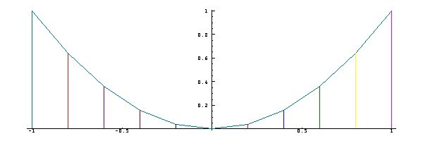 Similarly,
a
graph
of
the
cube
is
reflected
in
the
origin,
because
the
cube
of
Similarly,
a
graph
of
the
cube
is
reflected
in
the
origin,
because
the
cube
of
-x
equals
the
negative
of
the
cube
of
x:
cube=: ^ with 3
PLOT x;cube x
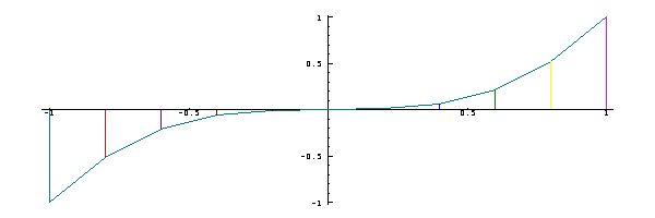
(cube -x)=(-cube x)
1 1 1 1 1 1 1 1 1 1 1
(sqr x)=(sqr x)
1 1 1 1 1 1 1 1 1 1 1
Simple
algebra
shows
that
for
any
function
f
,
the
function
ef=: f + f with -
is
even,
and
that
the
function
of=: f - f with -
is
odd.
For
example:
f=: ^ NB. The exponential (which is neither even nor odd)
ef=: f+f with -
of=: f-f with -
PLOT x;(f,ef,:of) x
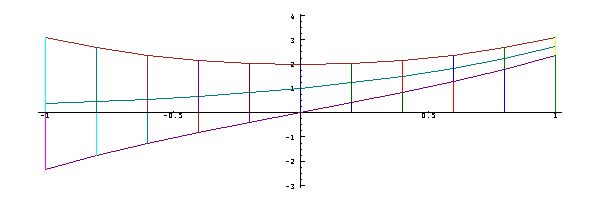 The
functions
The
functions
hef=: ef % 2:
and
hof=: of % 2:
are
called
the
even
and
odd
parts
of
f
because
they
are,
respectively,
even
and
odd,
and
because
they
sum
to
f:
hef=: ef % 2:
hof=: of % 2:
(f=hef+hof) x
1 1 1 1 1 1 1 1 1 1 1
PLOT x;(hef,hof,:hef+hof) x
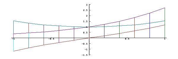 The
odd
and
even
parts
of
a
function
are
often
functions
of
interest
in
their
own
right.
For
example,
The
odd
and
even
parts
of
a
function
are
often
functions
of
interest
in
their
own
right.
For
example,
hof
is
the
hyperbolic
sine,
and
hef
is
the
hyperbolic
cosine.
They
are
denoted
in
J
by
5 with o.
and
6 with o.,
respectively.
15A.
Dot
product
and
vector
functions
15A.
Dot
product
and
vector
functions
S15A.
The
expression
+/w*x
gives
a
sum
over
the
argument
x
weighted
by
the
vector
w.
For
example:
x=: 2 3 5 7 11
w=: 0 1 2 3 4
w*x
0 3 10 21 44
+/w*x
78
The
dot
operator
(.)
applied
to
the
functions
+/
and
*
produces
an
equivalent
function
called
the
dot,
inner,
or
matrix
product.
Thus:
dp=: +/ . *
w dp x
78
Moreover,
dp
applies
to
a
matrix
(table)
left
argument
to
produce
a
vector
(list)
of
results,
using
successive
rows
of
the
matrix
as
weights.
For
example:
a=: 3 1 4
b=: 2 7 8
c=: 2 1 0
]m=: a,b,:c
3 1 4
2 7 8
2 1 0
m dp 2 3 5
29 65 7
b dp 2 3 5
65
g=: m with dp
g 2 3 5
29 65 7
If
m
is
a
square
matrix
(as
in
the
present
example),
then
m with dp
applies
to
a
vector
to
produce
a
vector
of
the
same
number
of
elements.
We
will
call
such
a
function
a
vector
function.
15B.
Dot
product
as
a
linear
vector
function
S15B.
The
dot
product
with
a
vector
or
matrix
left
argument
distributes
over
addition,
and
is
therefore
a
linear
function,
as
defined
in
Section
14F.
For
example:
x=: 2 3 5
y=: 0 1 2
f=: 2 7 8 with dp
((f x)+(f y)) , (f x+y)
88 88
g=: m with dp
((g x)+(g y)) ,: (g x+y)
38 88 8
38 88 8
The
function
I=: =/~ on i.
yields
a
result
called
an
identity
matrix,
because
when
used
with
dp
it
produces
an
identity
function
(that
yields
its
argument
unchanged).
For
example:
I=: i. =/ i.
]i=: I 3
1 0 0
0 1 0
0 0 1
i with dp 2 3 5
2 3 5
A
linear
vector
function
need
not
be
expressed
as
a
dot
product,
but
if
it
is
not,
the
required
matrix
is
easily
determined.
For
example,
sop=: +/\
(sums
over
prefixes)
is
a
linear
vector
function,
and
the
matrix
m
for
an
equivalent
function
m with dp
may
be
determined
as
follows:
x=: 2 3 5 7 11
y=: 0 1 2 3 4
sop=: +/\
((sop x)+(sop y)) ,: (sop x+y)
2 6 13 23 38
2 6 13 23 38
]i=: I # x
1 0 0 0 0
0 1 0 0 0
0 0 1 0 0
0 0 0 1 0
0 0 0 0 1
i dp x
2 3 5 7 11
sop i dp x
2 5 10 17 28
(sop i) dp x
2 5 10 17 28
]m=: sop i
1 0 0 0 0
1 1 0 0 0
1 1 1 0 0
1 1 1 1 0
1 1 1 1 1
The
resulting
matrix
provides
an
interesting
way
of
looking
at
the
sums
over
prefixes:
the
ones
in
the
successive
rows
indicate
the
elements
included
in
the
successive
sums.
15C.
Matrix
inverse
S15C.
The
inverse
of
a
linear
vector
function
m with dp
is
itself
a
linear
vector
function,
and
can
therefore
be
expressed
in
the
form
mi with dp.
The
matrix
mi
may
be
obtained
from
m
by
applying
the
matrix
inverse
function
%.
.
Thus:
]z=: m dp x=: 2 3 5 7 11
2 5 10 17 28
mi=: %.m
mi dp z
2 3 5 7 11
mi
1 0 0 0 0
_1 1 0 0 0
0 _1 1 0 0
0 0 _1 1 0
0 0 0 _1 1
The
pairs
_1 1
in
the
rows
of
the
inverse
mi
indicate
that
the
inverse
of
the
sum
over
prefixes
is
a
differencing
operation,
and
the
matrix
mi
may
be
called
a
difference
matrix.
|.),
rotation
(2 with |.)
and
8 with A..
16A.
Ascending
and
descending
order
of
exponents
16A.
Ascending
and
descending
order
of
exponents
S16A.
In
conventional
mathematics,
polynomials
are
sometimes
expressed
with
the
exponents
in
ascending
order
(beginning
with
zero),
and
sometimes
in
descending
order
(beginning
with
the
largest
exponent).
Thus:
pa
(for
ascending
order),
and
pd
(for
descending).
The
former
is
the
function
p.
that
we
have
used
in
earlier
chapters,
and
the
latter
may
be
expressed
in
terms
of
it
using
the
reversal
function
(|.)
to
reverse
the
order
of
the
coefficients.
Thus:
pa=: p.
pd=: |. on [ pa ]
x=: 0 1 2 3 4 5
1 2 3 pa x
1 6 17 34 57 86
1 2 3 pd x
3 6 11 18 27 38
1 2 3 pd 10
123
10
gives
the
value
in
decimal
of
the
digits
in
the
list
of
coefficients.
In
fact,
the
decimal
number
system
(and
number
systems
with
bases
other
than
ten)
are
"polynomial
representations"
of
numbers,
and
we
may
find
that
schemes
for
multiplying
polynomials
lead
to
improved
methods
of
multiplying
multi-digit
decimal
numbers.
16B.
Products
of
polynomials
S16B.
The
product
of
two
polynomials
c1 with p.
and
c2 with p.
is
itself
a
polynomial,
whose
coefficients
can
be
computed
from
c1
and
c2
by
first
forming
their
multiplication
table.
For
example:
c1=: 2 3 5
c2=: 4 1 0 3
c1 * table c2
+-+---------+
| | 4 1 0 3|
+-+---------+
|2| 8 2 0 6|
|3|12 3 0 9|
|5|20 5 0 15|
+-+---------+
The
coefficient
8
in
the
upper
left
corner
is
the
coefficient
of
x^0
in
the
product
polynomial,
the
elements
of
the
next
diagonal
(2 12)
are
coefficients
of
x^1,
the
next
diagonal
has
coefficients
of
x^2,
and
so
on.
The
combined
coefficients
of
successive
powers
may
therefore
be
obtained
by
summing
diagonals
of
the
table
to
obtain
c3=: 8 14 23 11 9 15.
Thus:
c3=: 8 14 23 11 9 15
x=: 0 1 2 3 4 5
(c1 p. x) * (c2 p. x)
8 80 840 4928 18800 54528
c3 p. x
8 80 840 4928 18800 54528
In
the
expression
f/.
the
oblique
operator
/.
produces
a
function
that
applies
f
to
each
of
the
diagonals
of
a
table
argument.
Thus:
c1 */ c2
8 2 0 6
12 3 0 9
20 5 0 15
+//. c1 */ c2
8 14 23 11 9 15
c3 = +//. c1 */ c2
1 1 1 1 1 1
We
may
therefore
define
a
function
pc
to
produce
product
coefficients
as
follows:
pc=: +//. on (*/)
c1 pc c2
8 14 23 11 9 15
1 1 pc 1 1
1 2 1
1 1 pc 1 1 pc 1 1
1 3 3 1
Similar
reasoning
will
show
that
the
same
function
pc
produces
coefficients
for
the
product
of
descending
polynomials.
This
may
be
tested
as
follows:
c1 pd x
5 10 19 32 49 70
c2 pd x
3 8 39 120 275 528
(c1 pd x)*(c2 pd x)
15 80 741 3840 13475 36960
c3 pd x
15 80 741 3840 13475 36960
16C.
Multiplication
of
decimal
numbers
S16C.
The
last
result
of
Section
16A
indicates
that
the
result
of
c pd 10
is
the
decimal
value
of
the
number
whose
digits
are
the
elements
of
the
list
c.
Thus:
c1=: 1 2 3
c2=: 1 2 0 3
(c1 pd 10),(c2 pd 10)
123 1203
c1 pc c2
represent
the
product
of
the
numbers
123
and
1203.
Thus:
]c3=: c1 pc c2
1 4 7 9 6 9
c3 pd 10
147969
123*1203
147969
Consequently,
the
product
can
be
obtained
by
making
the
table
c1 * table c2
and
summing
its
diagonals:
c1 * table c2
+-+-------+
| |1 2 0 3|
+-+-------+
|1|1 2 0 3|
|2|2 4 0 6|
|3|3 6 0 9|
+-+-------+
1,(+/2 2),(+/0 4 3),(+/3 0 6),(+/6 0),9
1 4 7 9 6 9
However,
these
diagonal
sums
for
other
arguments
may
yield
results
greater
than
9,
and
therefore
themselves
be
multi-digit
numbers.
For
example:
c4=: 1 2 3 4 5 6 7
c5=: 8 7 6 5 4
]c6=: c4 pc c5
8 23 44 70 100 130 160 126 92 59 28
c6 pd 10
108214735818
1234567*87654
108214735818
The
result
c6
does
correctly
represent
the
product,
but
it
is
unsatisfactory
in
that
its
multi-digit
elements
cannot
be
simply
squeezed
together
(as
in
8234470100130160126925928)
to
produce
the
correct
product.
c6=: 8 23 44 70 100 130 160 126 92 59 28
c7=: 8 23 44 70 100 130 160 126 92 61 8
c8=: 8 23 44 70 100 130 160 126 98 1 8
c9=: 8 23 44 70 100 130 160 135 8 1 8
c10=: 8 23 44 70 100 130 173 5 8 1 8
c11=: 8 23 44 70 100 147 3 5 8 1 8
c12=: 8 23 44 70 114 7 3 5 8 1 8
c13=: 8 23 44 81 4 7 3 5 8 1 8
c14=: 8 23 52 1 4 7 3 5 8 1 8
c15=: 8 28 2 1 4 7 3 5 8 1 8
c16=: 10 8 2 1 4 7 3 5 8 1 8
c17=: 1 0 8 2 1 4 7 3 5 8 1 8
c6 pd 10
108214735818
c17 pd 10
108214735818
Moreover,
the
entire
normalization
from
c6
to
c17
can
be
done
easily
by
hand
in
a
single
process.
In
summary,
multiplication
of
decimal
numbers
represented
by
the
lists
of
digits
d1
and
d2
can
be
performed
by
hand
by
writing
down
the
table
d1 * table d2,
summing
the
diagonals,
and
"normalizing"
the
results
to
single-digit
elements
(written
together
without
spaces).
This
process
may
be
compared
with
the
commonly-taught
scheme
shown
below:
1234567
87654
------------
4938268
6172835
7407402
8641969
9876536
------------
108214735818
In
contrast
to
the
three
distinct
steps
of
recording
the
multiplications
in
a
table,
summing
its
diagonals,
and
a
final
normalizion
by
carry,
this
conventional
scheme
combines
multiplication
and
carry
in
each
step
of
the
production
of
each
line,
and
again
uses
carrying
in
the
final
summation
of
the
several
lines.
16D.
Other
bases
S16D.
Just
as
c pd 10
gives
the
decimal
(or
base-10)
value
of
c
as
a
weighted
sum
with
weights
of
decreasing
powers
of
10,
so
c pd 8
gives
the
base-8
value,
using
powers
of
8
as
weights.
For
example:
c1=: 1 2 3
c2=: 1 2 0 3
(c1 pd 8),(c2 pd 8)
83 643
]c3=: c1 pc c2
1 4 7 9 6 9
c3 pd 8
53369
(c1 pd 8)*(c2 pd 8)
53369
Again
the
result
c3
can
be
normalized,
this
time
to
the
range
0
to
7.
This
requires
dividing
by
8,
"carrying"
the
integer
quotient,
and
leaving
the
remainder.
Thus:
c3
1 4 7 9 6 9
1 4 7 9 7 1 pd 8
53369
1 4 8 1 7 1 pd 8
53369
1 5 0 1 7 1 pd 8
53369
16E.
Remainder,
Divisibility,
and
Integer
part
S16E.
The
carrying
process
used
in
preceding
sections
made
use
of
the
remainder.
For
example,
8
divides
into
24
exactly
(that
is,
an
integer
number
of
times),
but
it
divides
27
leaving
a
remainder
of
3.
|
and
is
illustrated
by:
| table i=: 1 2 3 4 5 6 7 8
+-+---------------+
| |1 2 3 4 5 6 7 8|
+-+---------------+
|1|0 0 0 0 0 0 0 0|
|2|1 0 1 0 1 0 1 0|
|3|1 2 0 1 2 0 1 2|
|4|1 2 3 0 1 2 3 0|
|5|1 2 3 4 0 1 2 3|
|6|1 2 3 4 5 0 1 2|
|7|1 2 3 4 5 6 0 1|
|8|1 2 3 4 5 6 7 0|
+-+---------------+
d|n
is
zero,
we
say
that
n
is
divisible
by
d,
as
illustrated
by
the
following
divisibility
table:
=&0 on | table i
+-+---------------+
| |1 2 3 4 5 6 7 8|
+-+---------------+
|1|1 1 1 1 1 1 1 1|
|2|0 1 0 1 0 1 0 1|
|3|0 0 1 0 0 1 0 0|
|4|0 0 0 1 0 0 0 1|
|5|0 0 0 0 1 0 0 0|
|6|0 0 0 0 0 1 0 0|
|7|0 0 0 0 0 0 1 0|
|8|0 0 0 0 0 0 0 1|
+-+---------------+
n-d|n
is
divisible
by
d,
and
the
result
of
the
division
d%~n-d|n
is
called
the
integer
quotient.
Thus:
iq=: ([%~]-|)"0
8 iq 22 23 24 25 26 27
2 2 3 3 3 3
iq table i
+-+---------------+
| |1 2 3 4 5 6 7 8|
+-+---------------+
|1|1 2 3 4 5 6 7 8|
|2|0 1 1 2 2 3 3 4|
|3|0 0 1 1 1 2 2 2|
|4|0 0 0 1 1 1 1 2|
|5|0 0 0 0 1 1 1 1|
|6|0 0 0 0 0 1 1 1|
|7|0 0 0 0 0 0 1 1|
|8|0 0 0 0 0 0 0 1|
+-+---------------+
<.
to
the
result
of
division.
For
example:
i%5
0.2 0.4 0.6 0.8 1 1.2 1.4 1.6
<.i%5
0 0 0 0 1 1 1 1
<. on (%~) table i
+-+---------------+
| |1 2 3 4 5 6 7 8|
+-+---------------+
|1|1 2 3 4 5 6 7 8|
|2|0 1 1 2 2 3 3 4|
|3|0 0 1 1 1 2 2 2|
|4|0 0 0 1 1 1 1 2|
|5|0 0 0 0 1 1 1 1|
|6|0 0 0 0 0 1 1 1|
|7|0 0 0 0 0 0 1 1|
|8|0 0 0 0 0 0 0 1|
+-+---------------+
16F.
Notes
S16F.
In
his
Chapter
6:
The
Dawn
of
nothing,
Hogben
provides
an
interesting
discussion
of
number
systems
and
the
role
of
zero
in
their
development.
For
example:
Why
this
is
necessarily
true,
is
easy
to
see
if
we
recall
the
Roman
representation
of
32,
i.e.
XXXII.
If
the
Romans
had
written
it
in
the
form
III
II,
there
would
have
been
no
way
of
distinguishing
it
from
302,
320,
3,020,
3,200,
etc.
The
one
simple
way
of
escape
from
this
dilemma
is
to
introduce
a
sign
such
as
the
Maya
lozenge
...,
a
dot
or
a
circle
for
the
empty
column
of
the
abacus.
We
can
then
write
32,
302,
320,
3,020
as
below:
17A.
Introduction
17A.
Introduction
S17A.
In
cooking,
a
list
of
one
or
more
instructions
is
called
a
recipe;
in
mathematics
or
computer
science
it
is
called
a
program
or
algorithm.
odd=: 1:+even
even=: 2:*i.
odd
makes
use
of
the
function
even,
and
each
function
may
be
used
independently:
odd 5
1 3 5 7 9
even 5
0 2 4 6 8
(odd*even) 5
0 6 20 42 72
17B.
Designing
an
algorithm
S17B.
Except
for
the
very
simplest
cases,
it
is
best
to
begin
by
computing
an
example
and
assessing
its
suitability,
and
only
then
composing
the
required
definition
or
definitions.
We
will
illustrate
two
approaches
to
this
final
step:
f
and
g),
and
use
them
in
a
single
definition
(such
as
h=: f+f on g).
x.
and
y.
.
x,
and
applying
sine
and
decay
functions
to
it:
x=: 1r2*i.11
s=: 1&o. x
]n=: _1r5 * x
0 _1r10 _1r5 _3r10 _2r5 _1r2 _3r5 _7r10 _4r5 _9r10 _1
d=: ^ n
set 2
d*s
0 0.43 0.69 0.74 0.61 0.36 0.077 _0.17 _0.34 _0.4 _0.35
PLOT x;d,s,:d*s
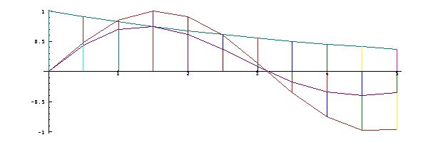
17C.
Explicit
definition
S17C.
We
will
now
illustrate
the
use
of
a
form
of
definition
in
which
the
arguments
occur
explicitly
(using
the
names
x.
and
y.),
and
allows
multiple
lines
in
which
names
may
be
assigned
to
intermediate
results.
Thus:
b=: 4
b
4
f=: 4 : 0
a=: i. x.
b=: a ^ y.
c=: +/b
b;c
)
5 f 2
+----------+--+
|0 1 4 9 16|30|
+----------+--+
b
0 1 4 9 16
It is clear that the value originally assigned to b
(in
order
to
illustrate
this
matter)
has
been
changed
by
the
execution
of
f,
behaviour
that
might
cause
the
loss
of
valuable
data.
This
unsuitable
behaviour
can
be
avoided
by
using
a
different
copula
(=.)
to
localize
the
names
assigned
within
the
function.
Thus:
f=: 4 : 0
a=.i. x.
b=.a ^ y.
c=.+/b
b;c
)
7 f 3
+-------------------+---+
|0 1 8 27 64 125 216|441|
+-------------------+---+
b
0 1 4 9 16
See
Section
S16C
for
a
further
example
of
explicit
definition.
@.
was
used
to
provide
a
conditional
execution
of
functions
in
its
argument.
In
many
programming
languages,
conditional
execution
is
provided
by
constructs
such
as
if,
then,
else,
and
while
do.
The
form
used
in
explicit
definition
is
illustrated
by:
SUM=: 3 : 0
i=.0
a=.0
while. i<y.
do. a=.next a
i=.next i
end.
a
)
SUM 4
6
0+1+2+3
6
sum=: +/ on i.
sum 4
6
18A.
Introduction
18A.
Introduction
S18A.
Just
as
the
operator
d.1
can
be
applied
to
a
function
f
to
obtain
its
derivative,
so
the
operator
d._1
can
be
applied
to
obtain
its
anti-derivative,
that
is,
a
function
whose
derivative
is
f.
For
example:
derv=: d.1
anti=: d._1
c=: 1 2 3 4 5 6
c with p.
1 2 3 4 5 6&p.
c with p. derv
2 6 12 20 30&p.
c with p. anti
0 1 1 1 1 1 1&p.
c with p. anti derv
1 2 3 4 5 6&p.
derv
and
anti
on
functions
such
as
^
and
1&o.
and
2&o.
and
6&o.
1 2 3 4 5&p.
and
7 2 3 4 5&p. ,
and
explain
their
agreement.
18B.
Area
under
a
graph
as
a
function
S18B.
A
study
of
the
graph
of
Section
3B
(an
approximation
to
a
circle)
suggests
that
the
area
under
the
graph
of
a
function
f
from
the
argument
_1
(or
any
fixed
point)
to
an
argument
x
is
itself
a
function
of
x
(that
depends
upon
the
function
f).
a=: i:1j40
PLOT a;cir a
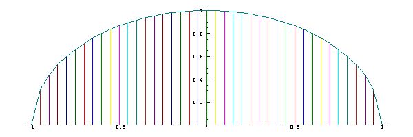 What
is
the
rate
of
change
of
the
area
function?
What
is
the
rate
of
change
of
the
area
function?
x=: 0.5,
the
spacing
s=: 0.05,
and
the
next
plotted
point
x+s.
The
change
in
area
is
due
to
the
quadrilateral
with
base
s
and
heights
cir x
and
cir x+s,
an
area
equal
to
s
times
the
average
of
the
heights
cir x
and
cir x+s.
((cir x+s)-(cir x))%s
is
therefore
the
average
of
cir x
and
cir x+s.
For
small
values
of
s,
this
average
approaches
cir x;
the
derivative
of
the
area
under
the
graph
of
cir
is
therefore
the
function
cir
itself.
18C.
Polynomial
approximations
S18C.
As
illustrated
in
Section
3B,
the
area
under
a
curve
can
be
computed
to
give
the
value
of
the
anti-derivative
of
a
function
at
a
chosen
point.
But
this
does
not
yield
a
function
for
the
anti-derivative
in
the
sense
that
the
operator
d._1
does
for
the
functions
to
which
it
applies.
f
is
provided
by
finding
the
coefficients
of
a
polynomial
that
approximates
it,
and
then
using
the
fact
that
the
anti-derivative
(as
well
as
the
derivative)
of
a
polynomial
is
easily
obtained.
(f x) %. x^/i.n
yields
the
coefficients
of
an
n-term
polynomial
that
best
fits
the
function
f
at
the
points
x.
For
example:
]x=: i:1j10
_1 _0.8 _0.6 _0.4 _0.2 0 0.2 0.4 0.6 0.8 1
]c=: (1&o. x) %. x ^/i.5
_3.46945e_17 0.997542 9.99201e_16 _0.156378 _7.77156e_16
c&p. _1 0 1
_0.841164 _3.46945e_17 0.841164
1&o. _1 0 1
_0.841471 0 0.841471
(c&p. x) ,. (sin x)
_0.841164 _0.841471
_0.717968 _0.717356
_0.564748 _0.564642
_0.389009 _0.389418
_0.198257 _0.198669
_3.46945e_17 0
0.198257 0.198669
0.389009 0.389418
0.564748 0.564642
0.717968 0.717356
0.841164 0.841471
The
polynomial
approximations
may,
however,
be
wildly
wrong
for
arguments
outside
of
the
list
x
to
which
it
was
fitted.
der
of
Section
6B
applied
to
a
list
of
polynomial
coefficients
yields
the
coefficients
of
the
derivative
polynomial.
A
coresponding
function
for
the
anti-derivative
may
be
defined
as
follows:
der=: 1: |. ] * i. on #
ant=: 0:,] % next i. on #
ant c
0 1 1 1 1 1 1
der ant c
1 2 3 4 5 6 0
19A.
Imaginary
numbers
19A.
Imaginary
numbers
S19A.
In
Chapter
1
we
began
with
the
counting
numbers
(1 2 3 4
etc.)
and
found
that
the
introduction
of
subtraction
as
the
inverse
of
addition
led
to
a
new
class
of
negative
numbers
(when
we
attempted
to
subtract
a
larger
number
from
a
smaller).
set=: 9!:11
set 4
sqr=: *:
sqrt=: sqr^:_1
a=: i.10
a
0 1 2 3 4 5 6 7 8 9
sqr a
0 1 4 9 16 25 36 49 64 81
sqrt a
0 1 1.414 1.732 2 2.236 2.449 2.646 2.828 3
b=: sqrt -a
b
0 0j1 0j1.414 0j1.732 0j2 0j2.236 0j2.449 0j2.646 0j2.828 0j3
sqr b
0 _1 _2 _3 _4 _5 _6 _7 _8 _9
19B.
Complex
numbers
S19B.
The
sum
of
a
real
and
an
imaginary
number
is
called
a
complex
number.
For
example:
a+b
0 1j1 2j1.414 3j1.732 4j2 5j2.236 6j2.449 7j2.646 8j2.828 9j3
sqr (a+b)
0 0j2 2j5.657 6j10.39 12j16 20j22.36 30j29.39 42j37.04 56j45.25 72j54
a + table b
+-+-------------------------------------------------------------+
| |0 0j1 0j1.414 0j1.732 0j2 0j2.236 0j2.449 0j2.646 0j2.828 0j3|
+-+-------------------------------------------------------------+
|0|0 0j1 0j1.414 0j1.732 0j2 0j2.236 0j2.449 0j2.646 0j2.828 0j3|
|1|1 1j1 1j1.414 1j1.732 1j2 1j2.236 1j2.449 1j2.646 1j2.828 1j3|
|2|2 2j1 2j1.414 2j1.732 2j2 2j2.236 2j2.449 2j2.646 2j2.828 2j3|
|3|3 3j1 3j1.414 3j1.732 3j2 3j2.236 3j2.449 3j2.646 3j2.828 3j3|
|4|4 4j1 4j1.414 4j1.732 4j2 4j2.236 4j2.449 4j2.646 4j2.828 4j3|
|5|5 5j1 5j1.414 5j1.732 5j2 5j2.236 5j2.449 5j2.646 5j2.828 5j3|
|6|6 6j1 6j1.414 6j1.732 6j2 6j2.236 6j2.449 6j2.646 6j2.828 6j3|
|7|7 7j1 7j1.414 7j1.732 7j2 7j2.236 7j2.449 7j2.646 7j2.828 7j3|
|8|8 8j1 8j1.414 8j1.732 8j2 8j2.236 8j2.449 8j2.646 8j2.828 8j3|
|9|9 9j1 9j1.414 9j1.732 9j2 9j2.236 9j2.449 9j2.646 9j2.828 9j3|
+-+-------------------------------------------------------------+
Since
a
complex
number
is
a
sum
of
a
real
and
an
imaginary
number,
the
product
of
complex
numbers
is
treated
consistently
as
a
product
of
sums.
The
steps
in
the
multiplication
may
be
illustrated
as
follows:
c=: 2j3
d=: 4j5
c*d
_7j22
(2+0j3)*(4+0j5)
_7j22
(2*(4+0j5))+(0j3*(4+0j5))
_7j22
(2*4)+(2*0j5)+(0j3*4)+(0j3*0j5)
_7j22
8+0j10+0j12+_15
_7j22
_7+0j22
_7j22
Note
that
the
product
of
two
imaginaries
(0j3
and
0j5)
yields
a
negative
real
number.
19C.
Division
S19C.
We
begin
by
dividing
the
product
e=: c*d
by
c
and
then
by
d
to
get
the
expected
results
d
and
c:
]e=: c*d
_7j22
e%c
4j5
e%d
2j3
To
get
a
general
procedure
for
division,
we
first
note
that
division
by
a
real
number
is
straightforward.
For
example:
12j22 % 2
6j11
Similarly,
we
note
that
multiplication
of
both
numerator
and
dednominator
by
the
same
number
leaves
the
quotient
unchanged.
For
example:
e%c
4j5
g=: 2j_3
(e*g)%(c*g)
4j5
Finally,
we
note
that
the
denominator
c*g
is
a
real
number,
a
result
of
choosing
g
as
the
conjugate
of
c,
that
is,
obtained
from
c
by
reversing
the
sign
of
its
imaginary
part:
c*g
13
The
function
conj=: +
yields
the
conjugate
of
its
argument,
and
it
can
therefore
be
used
to
provide
division
by
first
producing
an
equivalent
quotient
with
a
real
denominator.
For
example:
conj=: +
p=: 2j5
q=: 3j_4
p%q
_0.56j0.92
conj q
3j4
p*conj q
_14j23
q*conj q
25
(p*conj q)%(q*conj q)
_0.56j0.92
NB. Compare with p%q
19D.
The
Exponential
Family
S19D.
In
Chapter
14
we
showed
that
the
hyperbolic
sine
and
the
hyperbolic
cosine
belonged
to
the
exponential
family
in
the
sense
that
they
could
be
obtained
from
the
exponential
as
its
odd
and
even
parts.
Using
imaginary
numbers,
we
can
treat
the
sine
and
cosine
similarly.
j.
multiplies
its
argument
by
0j1
(the
square
root
of
negative
one).
For
example:
j.i.10
0 0j1 0j2 0j3 0j4 0j5 0j6 0j7 0j8 0j9
Consequently,
each
term
in
the
polynomial
c with p. on j.
differs
from
that
in
the
polynomial
c with p.
by
a
power
of
0j1
determined
by
its
exponent.
For
example:
0j1^0 1 2 3 4 5 6 7 8
1 0j1 _1 0j_1 1 0j1 _1 0j_1 1
c=: 1 2 3 4 5 6 7
f=: c with p.
f t. i.10 NB. Taylor coefficients
1 2 3 4 5 6 7 0 0 0
f on j. t. i.10
1 0j2 _3 0j_4 5 0j6 _7 0 0 0
Consequently,
the
Taylor
coefficients
of
the
function
^ with j.
are
the
same
as
those
of
the
sum
cos+j. sin,
and
the
cosine
and
sine
can
be
obtained
from
the
even
and
odd
parts
of
^ with j.
O=: .: -
E=: .. -
and experiment with their use on the function
f=: 0 1 2 3 4 5 with p.
using
expressions
such
as
f E
and
f E i:4
and
(f O+f E) i:4
^
and
sin=: 1 with o.
and
cos=: 2 with o.
and
cosh=: 6 with o. .
20A.
Introduction
20A.
Introduction
S20A.
In
stating
the
purpose
of
this
book
in
the
preface
we
said:
In
the
seventy-odd
years
since
his
publication,
the
development
of
computer
programming
has
provided
languages
with
grammars
that
are
simpler
and
more
tractable
than
that
of
conventional
mathematical
notation.
Moreover,
the
general
availability
of
the
computer
makes
possible
convenient
and
accurate
experimentation
with
mathematical
ideas....
The
unstated
premise
of
this
book
-
a
premise
that
virtually
all
mathematicians
would
agree
to
-
is
that
mathematics,
like
music,
is
worth
doing
for
its
own
sake.
The
author
is,
by
profession,
a
medical
man,
but
he
has
a
love
for
mathemtics
and
wants
others
to
share
his
enthusiasm.
The
course
title
"Concrete
Mathematics"
was
originally
intended
as
an
antidote
to
"Abstract
Mathematics",
since
concrete
classical
results
were
rapidly
being
swept
out
of
the
modern
mathematical
curriculum
by
a
new
wave
of
abstract
ideas
popularly
called
"The
New
Math."
Abstract
mathematics
is
a
beautiful
subject
...
But
its
adherents
had
become
deluded
that
the
rest
of
mathematics
was
inferior
and
no
longer
worthy
of
attention.
20B.
Mathematics:
from
the
Birth
of
Numbers
S20B.
We
will
comment
on
four
topics
covered
by
Gullberg,
primarily
to
show
the
form
of
their
expression
in
J,
and
the
possibility
for
computer
experimentation:
All real numbers can be written as periodic
or nonperiodic, terminating or nonterminating, decimal
fractions. Another way of writing a rational number
is in the form of a continued fraction,
This
is
equivalent
to
the
function
pr=: [+1:%]
applied
over
the
list
a0,a1,a2,a3, etc.,
and
Gullberg's
example
of
221/41
may
be
treated
as
follows:
pr=: [+1:%]
2 pr 5
2.2
pr/5 2 1 1 3 2r1
221r41
pr/5 2 1 1 3 2
5.39024
pr/\5 2 1 1 3 2r1
5 11r2 16r3 27r5 97r18 221r41
The
final
expression
illustrates
how
the
operator
\
may
be
used
to
obtain
the
partial
sums
or
"convergents"
to
the
complete
continued
fraction.
pr/\1 1 1 1 1 1 1 1 1 1r1
1 2 3r2 5r3 8r5 13r8 21r13 34r21 55r34 89r55
pr/\1 1 1 1 1 1 1 1 1 1
1 2 1.5 1.66667 1.6 1.625 1.61538 1.61905 1.61765 1.61818
These
decimal
results
may
be
recognized
as
increasingly
good
approximations
to
the
Golden
Mean
(or
golden
number),
also
treated
by
Gullberg.
a=: 2 2 4 2 4 2 4 2 4
b=: pr/a
b
2.44949
b*b
6
DETERMINANTS
On
pages
646,7,
Gullberg
states:
A determinant is a value
representing sums and products of a square matrix.
The determinant of a matrix A, det A, is denoted as
arrays of numbers or algebraic quantities, called
entries or elements, disposed in horizontal rows and
vertical columns enclosed between single vertical bars:
| a11 a12 ... a1n |
det A = | ... ... ... ... |
| an1 an2 ... ann |
...
has 3! = 6 triple products of entries from every row
and column, of which no two triplets can be the same,
a11 a22 a33 a11 a23 a32 a12 a21 a33 a12 a23 a31 a13 a21 a32 a13 a22 a31
1-2-3 1-3-2 2-1-3 2-3-1 3-1-2 3-2-1
# of inversions:
none one one two two three
Correction factor:
+1 -1 -1 +1 +1 -1
In
J
the
determinant
function
is
defined
as
det=: -/ . *
which,
applied
to
the
three-by-three
matrix
(that
is,
table)
of
Gullberg's
example
yields
the
following
results:
det=: -/ . *
A=: 2 3 4,.0 1 2,.4 0 2
A
2 0 4
3 1 0
4 2 2
det A
12
Gullberg
notes
the
following
properties:
The
value
of
a
determinant
is
reversed
in
sign
if
any
two
rows
are
interchanged.
For
example:
(1 A. A);(det 1 A. A);(det A)
+-----+---+--+
|2 0 4| | |
|4 2 2|_12|12|
|3 1 0| | |
+-----+---+--+
(1 3 1 * A);(det 1 3 1 * A);(3 * det A)
+-----+--+--+
|2 0 4| | |
|9 3 0|36|36|
|4 2 2| | |
+-----+--+--+
(2 3 4 * A);(det 2 3 4 * A);((*/2 3 4)*det A)
+------+---+---+
| 4 0 8| | |
| 9 3 0|288|288|
|16 8 8| | |
+------+---+---+
triangle=: 3 2$3 _2 , _4 1 , 8 3
bt=: triangle,.1
triangle;bt;(det bt);(1 A. bt);(det 1 A. bt)
+-----+-------+---+-------+--+
| 3 _2| 3 _2 1| | 3 _2 1| |
|_4 1|_4 1 1|_50| 8 3 1|50|
| 8 3| 8 3 1| |_4 1 1| |
+-----+-------+---+-------+--+
The
last
result
agrees
with
Gullberg's
statement
that
the
absolute
value
of
the
determinant
yields
twice
the
area
of
the
triangle.
But,
more
generally,
the
determinant
yields
a
signed
area
that
indicates
whether
the
vertices
of
the
triangle
(when
plotted)
occur
in
clockwise
or
counter-clockwise
order.
!3)
its
signed
volume.
For
example:
]tet=: 4 3$0 0 0 , 1 0 0 , 0 1 0 , 0 0 1
0 0 0
1 0 0
0 1 0
0 0 1
det tet,.1
_1
]tet2=: ?. 4 3$10
1 7 4
5 2 0
6 6 9
3 5 8
det tet2,.1
_106
LOGARITHMS
On
page
154
Gullberg
says:
that
is,
a
logarithm
is
an
exponent
which
defines
to
what
power
the
base
a
must
be
raised
in
order
to
give
x,
called
the
anti-logarithm.
In
J
the
function
a with ^.
gives
the
base
a
logarithm,
and
the
function
^.
(or
1x1 with ^.)
gives
the
natural
log.
Hence:
ln=: ^.
log=: 10 with ^.
lb=: 2 with ^.
x=: 1 2 4 10 100
ln x
0 0.693147 1.38629 2.30259 4.60517
log x
0 0.30103 0.60206 1 2
lb x
0 1 2 3.32193 6.64386
ln -1 2 4 10
0j3.14159 0.693147j3.14159 1.38629j3.14159 2.30259j3.14159
^ ln -x
_1 _2 _4 _10 _100
log -x
0j1.36438 0.30103j1.36438 0.60206j1.36438 1j1.36438 2j1.36438
10 ^ log -x
_1 _2 _4 _10 _100
THE
PEANO
AXIOMS
On
page
157
Gullberg
says:
The
natural
numbers
were
axiomatically
defined
in
1899
by
Giuseppe
Peano
in
his
...
Later,
Peano
modified
his
axioms
to
include
also
zero:
The
treatment
in
our
Chapter
1
is
based
on
Peano's
original
formulation
(which
did
not
include
zero
as
a
natural
number),
and
denotes
Peano's
successor
function
by
>:
(and
its
inverse,
the
predecessor,
by
<:).
20C.
Concrete
Mathematics
S20C.
The
text
Concrete
Mathematics
[2]
will
be
referred
to
as
GKP,
and
will
be
discussed
together
with
commentary
on
it
(expressed
in
J)
from
Concrete
Math
Companion
[21],
to
be
referred
to
as
CMC.
Our
generic
generating
function
has
the
form
In
Section
7B,
CMC
discusses
this
as
follows:
In
GKP7.12
the
limit
(as
SUBSCRIPTS
VERSUS
FUNCTIONS
In
Section
2.1
GKP
states
that:
n
approaches
infinity)
of
the
polynomial
G=. (g i.n) p. ]
is
defined
to
be
the
generating
function
for
the
function
g.
In
other
words,
g k
is
the
kth
element
of
the
Taylor
series
for
g.
gex=. ^ t.
gsin=. 1&o. t.
gsinex=. (1&o. * ^) t.
]ce=. gex i. 8
1 1 0.5 0.166667 0.0416667 0.00833333 0.00138889 0.000198413
]cs=. gsin i.8
0 1 0 _0.166667 0 0.00833333 0 _0.000198413
]cse=. gsinex i. 8
0 1 1 0.333333 0 _0.0333333 _0.0111111 _0.0015873
We'll
be
working
with
sums
of
the
general
form
In
Section
2A,
CMC
discusses
this
as
follows:
We
will
therefore
treat
STIRLING
NUMBERS
In
Section
6.1,
GKP
defines
Stirling
Numbers
of
the
first
and
second
kind
by:
a
as
a
function,
and
the
list
of
indices
as
a
second
function,
typically
i.
or
the
function
Ei=. i.@>: .
For
example
Ei=. i.@>:
Ei 5
0 1 2 3 4 5
a=. *:
a Ei 5
0 1 4 9 16 25
+/ a Ei 5
55
...the
number
of
ways
to
arrange
n
objects
into
k
cycles
and
provides
tables
of
them
in
Table
245
and
Table
244.
^!._1
and
uses
it
to
define
the
Stirling
numbers
as
matrices
that
provide
the
coefficients
for
linear
transformations
between
the
coefficients
of
certain
important
polynomials.
s1=: |: on ((i. ^!._1/ i.) %. (i. ^/ i.))
s2=: %. on s1
(s1;s2) 8r1
+--------------------------------+-----------------------+
|1 0 0 0 0 0 0 0|1 0 0 0 0 0 0 0|
|0 1 0 0 0 0 0 0|0 1 0 0 0 0 0 0|
|0 _1 1 0 0 0 0 0|0 1 1 0 0 0 0 0|
|0 2 _3 1 0 0 0 0|0 1 3 1 0 0 0 0|
|0 _6 11 _6 1 0 0 0|0 1 7 6 1 0 0 0|
|0 24 _50 35 _10 1 0 0|0 1 15 25 10 1 0 0|
|0 _120 274 _225 85 _15 1 0|0 1 31 90 65 15 1 0|
|0 720 _1764 1624 _735 175 _21 1|0 1 63 301 350 140 21 1|
+--------------------------------+-----------------------+
Functions
to
provide
Tables
245
and
244
of
GkP
are
defined
in
terms
of
these
as
follows
S1=: | on s1
S2=: s2
(S1;S2) 8r1
+----------------------------+-----------------------+
|1 0 0 0 0 0 0 0|1 0 0 0 0 0 0 0|
|0 1 0 0 0 0 0 0|0 1 0 0 0 0 0 0|
|0 1 1 0 0 0 0 0|0 1 1 0 0 0 0 0|
|0 2 3 1 0 0 0 0|0 1 3 1 0 0 0 0|
|0 6 11 6 1 0 0 0|0 1 7 6 1 0 0 0|
|0 24 50 35 10 1 0 0|0 1 15 25 10 1 0 0|
|0 120 274 225 85 15 1 0|0 1 31 90 65 15 1 0|
|0 720 1764 1624 735 175 21 1|0 1 63 301 350 140 21 1|
+----------------------------+-----------------------+
20D.
Computer
Resources
S20D.
LABORATORIES
Clicking
the
mouse
on
the
menu
item
marked
"Studio"
shows
a
menu
that
allows
the
selection
of
either
"Labs"
or
"Demos".
Clicking
on
"Labs"
provides
an
opportunity
to
choose
a
variety
of
topics.
,1,
produces
a
matrix
with
an
interesting
pattern.
Moreover,
it
provides
a
function
viewmat
that
plots
a
view
of
the
matrix
as
a
grid
of
black
and
white
elements.
Thus:
f=: ,~ ,.~
f ,1
1 1
1 0
f f ,1
1 1 1 1
1 0 1 0
1 1 0 0
1 0 0 0
f f f ,1
1 1 1 1 1 1 1 1
1 0 1 0 1 0 1 0
1 1 0 0 1 1 0 0
1 0 0 0 1 0 0 0
1 1 1 1 0 0 0 0
1 0 1 0 0 0 0 0
1 1 0 0 0 0 0 0
1 0 0 0 0 0 0 0
load 'graph numeric trig'
viewmat f f f f f f f f ,1
o.
will
show
that
the
definition
of
the
function
0 with o.
(used
to
graph
circles
in
Sections
3B
and
18B)
is
the
square
root
of
one
minus
the
square.
20E.
Conclusion
S20E.
Study
of
this
book
will
not
make
a
mathematician,
but
we
hope
that
the
use
of
precise
executable
language
possessing
a
simple
strict
grammar
will
further
the
cause
stated
by
Hogben
in
our
preface
(and
repeated
here):
Perhaps
the
most
important
lesson
for
the
layman
is
that
there
is
no
need
to
be
intimidated
by
mathematics
or
mathematicians.
On
this
matter,
we
give
the
final
word
to
Hogben:
There
is
a
story
about
Diderot,
the
Encyclopaedist
and
materialist,
a
foremost
figure
in
the
intellectual
awakening
which
immediately
preceded
the
French
Revolution.
Diderot
was
staying
at
the
Russian
court,
where
his
elegant
flippancy
was
entertaining
the
nobility.
Diderot
was
informed
that
a
mathematician
had
established
a
proof
of
the
existence
of
God.
a+bn
------- = x, donc Dieu existe, repondez!
n
Algebra
was
Arabic
to
Diderot.
Unfortunately,
he
did
not
realize
that
was
the
trouble.
Had
he
realized
that
algebra
was
just
a
language
in
which
we
describe
the
sizes
of
things,
...
he
would
have
asked
Euler
to
translate
...
into
French.
S1A.
The
Counting
(Natural)
Numbers
This
definition
of
the
counting
numbers
in
terms
of
a
successor
function
was
made
in
1899
by
Giuseppe
Peano.
For
further
details,
see
the
discussion
in
Section
20B,
and
the
Gullberg
text
to
which
it
refers.
S1B.
Lists
and
Names
The
function
(or
verb)
denoted
by
,.
can
be
used
to
stitch
lists
together
to
form
tables,
and
lists
and
tables
together
to
form
further
tables,
as
illustrated
by
the
following:
a=:1 4 7
b=:2 5 8
c=:3 6 9
a,.b
1 2
4 5
7 8
a,.b,.c
1 2 3
4 5 6
7 8 9
table=:a,.b,.c
table,.>:c
1 2 3 4
4 5 6 7
7 8 9 10
>:table
2 3 4
5 6 7
8 9 10
table,.>:>:>:table
1 2 3 4 5 6
4 5 6 7 8 9
7 8 9 10 11 12
The
function
denoted
by
,
can
be
used
to
catenate
lists
and
tables
as
illustrated
by
the
following:
a,b
1 4 7 2 5 8
a,b,c
1 4 7 2 5 8 3 6 9
table,a
1 2 3
4 5 6
7 8 9
1 4 7
table,>:>:>:>:>:>:>:>:>:table
1 2 3
4 5 6
7 8 9
10 11 12
13 14 15
16 17 18
The
function
denoted
by
|:
can
be
used
to
transpose
a
table
as
follows:
|:table
1 4 7
2 5 8
3 6 9
|:table,>:c
1 4 7 4
2 5 8 7
3 6 9 10
Write
various
expressions
employing
the
functions
used
in
the
preceding
examples,
and
show
the
results
produced.
S1C.
Iteration
(Repetition)
Write
the
result
of
the
expression
next for list list ,
and
compare
your
result
with
that
produced
by
entering
it
on
the
computer.
S1D.
Inverse
While
we
had
only
the
counting
numbers
(which
begin
at
1),
our
lists
could
contain
neither
negative
numbers
nor
zero;
but
now
that
we
have
extended
our
domain
to
the
integers
this
restriction
is
removed.
We
may
therefore
introduce
the
functions
i.
and
i:
that
produce
lists
of
integers
as
illustrated
below:
i.5 NB. The first five non-negative integers
0 1 2 3 4
i:5 NB. The integers from _5 to 5
_5 _4 _3 _2 _1 0 1 2 3 4 5
In
the
foregoing
we
used
NB.
which
indicates
that
what
follows
it
is
a
note
or
comment
that
has
no
effect
on
the
meaning
of
the
preceding
sentence.
+:
doubles
its
argument.
For
example:
x=:i:5
x
_5 _4 _3 _2 _1 0 1 2 3 4 5
+:x
_10 _8 _6 _4 _2 0 2 4 6 8 10
double=:+:
double x
_10 _8 _6 _4 _2 0 2 4 6 8 10
y=:double for 2 x
y
_20 _16 _12 _8 _4 0 4 8 12 16 20
double for _1 y NB. Inverse of double
_10 _8 _6 _4 _2 0 2 4 6 8 10
double for _1 x
_2.5 _2 _1.5 _1 _0.5 0 0.5 1 1.5 2 2.5
Some
of
the
results
of
the
last
expression
are
not
integers.
Just
as
the
inverse
of
the
successor
function
led
us
out
of
the
domain
of
the
counting
numbers,
so
the
inverse
of
double
has
led
out
of
the
domain
of
integers
--
this
time
into
fractions
or
rationals.
These
matters
are
treated
further
in
Section
1J.
S1E.
Addition
and
Subtraction
(+
and
-)
Study
the
following
function
tables,
and
try
to
state
the
definitions
of
each
of
the
functions
denoted
by
= > <. <: |
and
!
a=:i.6
a
0 1 2 3 4 5
=table a
+-+-----------+
| |0 1 2 3 4 5|
+-+-----------+
|0|1 0 0 0 0 0|
|1|0 1 0 0 0 0|
|2|0 0 1 0 0 0|
|3|0 0 0 1 0 0|
|4|0 0 0 0 1 0|
|5|0 0 0 0 0 1|
+-+-----------+
(=table a),.(>table a),.(<.table a)
+-+-----------+-+-----------+-+-----------+
| |0 1 2 3 4 5| |0 1 2 3 4 5| |0 1 2 3 4 5|
+-+-----------+-+-----------+-+-----------+
|0|1 0 0 0 0 0|0|0 0 0 0 0 0|0|0 0 0 0 0 0|
|1|0 1 0 0 0 0|1|1 0 0 0 0 0|1|0 1 1 1 1 1|
|2|0 0 1 0 0 0|2|1 1 0 0 0 0|2|0 1 2 2 2 2|
|3|0 0 0 1 0 0|3|1 1 1 0 0 0|3|0 1 2 3 3 3|
|4|0 0 0 0 1 0|4|1 1 1 1 0 0|4|0 1 2 3 4 4|
|5|0 0 0 0 0 1|5|1 1 1 1 1 0|5|0 1 2 3 4 5|
+-+-----------+-+-----------+-+-----------+
(<:table a),.(|table a),.(!table a)
+-+-----------+-+-----------+-+------------+
| |0 1 2 3 4 5| |0 1 2 3 4 5| |0 1 2 3 4 5|
+-+-----------+-+-----------+-+------------+
|0|1 1 1 1 1 1|0|0 1 2 3 4 5|0|1 1 1 1 1 1|
|1|0 1 1 1 1 1|1|0 0 0 0 0 0|1|0 1 2 3 4 5|
|2|0 0 1 1 1 1|2|0 1 0 1 0 1|2|0 0 1 3 6 10|
|3|0 0 0 1 1 1|3|0 1 2 0 1 2|3|0 0 0 1 4 10|
|4|0 0 0 0 1 1|4|0 1 2 3 0 1|4|0 0 0 0 1 5|
|5|0 0 0 0 0 1|5|0 1 2 3 4 0|5|0 0 0 0 0 1|
+-+-----------+-+-----------+-+------------+
=
is
a
truth
function
that
compares
its
arguments
for
equality,
giving
1
if
the
relation
is
true,
and
0
if
it
is
false.
>
is
a
truth
function
called
greater
than.
<.
is
called
lesser-of
or
minimum.
<:
is
a
truth
function
called
less
than
or
equal.
|
is
remainder
on
dividing
by
the
left
argument.
!
is
the
binomial
coefficient
(m!n
is
the
number
of
different
ways
of
choosing
m
things
from
n
things).
This
table
is
commonly
shown
without
the
zeros,
and
called
Pascal's
Triangle.
S1F.
Bonding
Apply
the
bond
(with=:&)
to
some
of
the
functions
= < >. <: |
introduced
in
Section
S1E,
and
show
their
results.
Compare
your
results
with
the
following:
with=: &
a=:i:3
a
_3 _2 _1 0 1 2 3
= with 2 a
0 0 0 0 0 1 0
< with 2 a
1 1 1 1 1 0 0
<: with 2 a
1 1 1 1 1 1 0
<. with 2 a
_3 _2 _1 0 1 2 2
2 with | a
1 0 1 0 1 0 1
3 with | a
0 1 2 0 1 2 0
S1G.
Multiplication
or
Times
(*)
Comment
on
the
pattern
of
positive
and
negative
numbers
in
the
four
quadrants
defined
by
the
row
and
column
of
zeros
in
the
following
multiplication
table:
* table i:4
+--+-----------------------------+
| | _4 _3 _2 _1 0 1 2 3 4|
+--+-----------------------------+
|_4| 16 12 8 4 0 _4 _8 _12 _16|
|_3| 12 9 6 3 0 _3 _6 _9 _12|
|_2| 8 6 4 2 0 _2 _4 _6 _8|
|_1| 4 3 2 1 0 _1 _2 _3 _4|
| 0| 0 0 0 0 0 0 0 0 0|
| 1| _4 _3 _2 _1 0 1 2 3 4|
| 2| _8 _6 _4 _2 0 2 4 6 8|
| 3|_12 _9 _6 _3 0 3 6 9 12|
| 4|_16 _12 _8 _4 0 4 8 12 16|
+--+-----------------------------+
The
idea
of
multiplication
can
be
introduced
at
an
elementary
level
by
pictures
of
rectangles.
For
example:
a=:3 4 $ 1
a
1 1 1 1
1 1 1 1
1 1 1 1
,a
1 1 1 1 1 1 1 1 1 1 1 1
+/,a
12
+/a
3 3 3 3
+/+/a
12
b=:|:a
b
1 1 1
1 1 1
1 1 1
1 1 1
,b
1 1 1 1 1 1 1 1 1 1 1 1
+/,b
12
+/b
4 4 4
+/+/b
12
Discussion
of
the
notation
used
here
(such
as
$)
may
be
found
in
Sections
2E
and
2F.
1
used
above,
but
uses
dots:
c=: a { ' .'
c
....
....
....
|:c
...
...
...
...
c='.'
1 1 1 1
1 1 1 1
1 1 1 1
+/+/c='.'
12
Moreover,
he
draws
a
tied
bag
(rather
similar
to
&)
to
denote
an
unknown
quantity,
and
translates
to
algebraic
expressions
that
denote
unknowns
by
letters
such
as
x
and
y.
For
example:
g=:'&&...'
g
&&...
translates
to
2x+3.
g,g
&&...&&...
which
is
denoted
by
(2x+3)+(2x+3)
and
is
(pictorially)
equivalent
to
that
shown
above,
or
to
&&&&......
which,
in
turn,
translates
to
4x+6.
S1H.
Power
and
Exponent
See
Section
S1J
for
an
extension
of
the
power
table
to
negative
arguments.
S1I.
Monomials
and
Polynomials
(p.)
Write
various
expressions
using
the
polynomial
function
p.
and
show
the
results
they
produce.
Include
cases
with
negative
coefficients
and
negative
arguments,
and
compare
your
results
with
the
following:
b=:i:4
b
_4 _3 _2 _1 0 1 2 3 4
1 3 3 1 p. b
_27 _8 _1 0 1 8 27 64 125
_1 3 _3 1 p. b
_125 _64 _27 _8 _1 0 1 8 27
(b-1)^3
_125 _64 _27 _8 _1 0 1 8 27
1 _4 6 _4 1 p. b
625 256 81 16 1 0 1 16 81
(b-1)^4
625 256 81 16 1 0 1 16 81
S1J.
Division
(%)
Comment
on
the
pattern
in
the
rows
and
columns
of
the
division
table.
Then
make
a
division
table
for
both
positive
and
negative
arguments,
and
compare
your
results
with
the
following:
c=:i:5r1
c
_5 _4 _3 _2 _1 0 1 2 3 4 5
%table c
+--+------------------------------------------------+
| | _5 _4 _3 _2 _1 0 1 2 3 4 5|
+--+------------------------------------------------+
|_5| 1 5r4 5r3 5r2 5 __ _5 _5r2 _5r3 _5r4 _1|
|_4| 4r5 1 4r3 2 4 __ _4 _2 _4r3 _1 _4r5|
|_3| 3r5 3r4 1 3r2 3 __ _3 _3r2 _1 _3r4 _3r5|
|_2| 2r5 1r2 2r3 1 2 __ _2 _1 _2r3 _1r2 _2r5|
|_1| 1r5 1r4 1r3 1r2 1 __ _1 _1r2 _1r3 _1r4 _1r5|
| 0| 0 0 0 0 0 0 0 0 0 0 0|
| 1|_1r5 _1r4 _1r3 _1r2 _1 _ 1 1r2 1r3 1r4 1r5|
| 2|_2r5 _1r2 _2r3 _1 _2 _ 2 1 2r3 1r2 2r5|
| 3|_3r5 _3r4 _1 _3r2 _3 _ 3 3r2 1 3r4 3r5|
| 4|_4r5 _1 _4r3 _2 _4 _ 4 2 4r3 1 4r5|
| 5| _1 _5r4 _5r3 _5r2 _5 _ 5 5r2 5r3 5r4 1|
+--+------------------------------------------------+
Comment
on
the
patterns
in
the
following
extension
of
the
power
table
to
negative
arguments.
In
particular,
note
the
value
of
0^0
(which
may
have
surprised
you
in
the
power
table
in
Section
1H).
1
for
the
value
of
the
"indeterminate"
expression
0^0,
see
page
785
of
Gullberg
[20].
^table c
+--+-----------------------------------------------------+
| | _5 _4 _3 _2 _1 0 1 2 3 4 5|
+--+-----------------------------------------------------+
|_5|_1r3125 1r625 _1r125 1r25 _1r5 1 _5 25 _125 625 _3125|
|_4|_1r1024 1r256 _1r64 1r16 _1r4 1 _4 16 _64 256 _1024|
|_3| _1r243 1r81 _1r27 1r9 _1r3 1 _3 9 _27 81 _243|
|_2| _1r32 1r16 _1r8 1r4 _1r2 1 _2 4 _8 16 _32|
|_1| _1 1 _1 1 _1 1 _1 1 _1 1 _1|
| 0| _ _ _ _ _ 1 0 0 0 0 0|
| 1| 1 1 1 1 1 1 1 1 1 1 1|
| 2| 1r32 1r16 1r8 1r4 1r2 1 2 4 8 16 32|
| 3| 1r243 1r81 1r27 1r9 1r3 1 3 9 27 81 243|
| 4| 1r1024 1r256 1r64 1r16 1r4 1 4 16 64 256 1024|
| 5| 1r3125 1r625 1r125 1r25 1r5 1 5 25 125 625 3125|
+--+-----------------------------------------------------+
S1K.
Review
and
Supplement
Experiment
with
moving
around
in
the
text
as
follows:
S1L.
Notes
S2A.
Introduction
To
gain
further
familiarity
with
the
computer,
enter
some
of
the
expressions
from
the
supplemental
sections
for
Chapter
1.
S2B.
Number
of
places
The
!:
used
in
the
expression
set=:9!:11
to
define
the
function
for
setting
the
number
of
digits
displayed
is
called
the
foreign
conjunction,
because
it
concerns
matters
other
than
the
normal
verbs
such
as
+ *
and
%.
set.
Also
click
on
the
button
marked
>>
to
see
further
pages.
S2C.
Displays
Sawyer
[22]
emphasizes
the
use
of
trees
and
tables
for
insight,
and
introduces
an
interesting
non-numeric
table
as
follows:
In
the
Japanese
Hiragana
alphabet,
each
character
represents
a
sound
such
as
ka,
ru,
si,
or
o.
There
are
10
possible
beginnings
-
the
consonants
k,
s,
t,
n,
m,
y,
r,
w,
and
'blank';
...
The
ending
is
always
one
one
of
the
five
sounds
a,
e,
i,
o,
u.
How
many
characters
are
there
in
this
alphabet?
We
could
show
this
as
a
tree
with
10
branches
and
5
twigs
on
each
...
This
problem
could
equally
well
be
solved
by
the
rectangle
...
Beginnings=:' KSTNHMYRW'
Endings=:'aeiou'
{ Beginnings;Endings
+--+--+--+--+--+
| a| e| i| o| u|
+--+--+--+--+--+
|Ka|Ke|Ki|Ko|Ku|
+--+--+--+--+--+
|Sa|Se|Si|So|Su|
+--+--+--+--+--+
|Ta|Te|Ti|To|Tu|
+--+--+--+--+--+
|Na|Ne|Ni|No|Nu|
+--+--+--+--+--+
|Ha|He|Hi|Ho|Hu|
+--+--+--+--+--+
|Ma|Me|Mi|Mo|Mu|
+--+--+--+--+--+
|Ya|Ye|Yi|Yo|Yu|
+--+--+--+--+--+
|Ra|Re|Ri|Ro|Ru|
+--+--+--+--+--+
|Wa|We|Wi|Wo|Wu|
+--+--+--+--+--+
The
catalogue
function
({)
used
above
may
be
further
illustrated
as
follows:
{ 0 1 2;0 1 2;0 1 2
+-----+-----+-----+
|0 0 0|0 0 1|0 0 2|
+-----+-----+-----+
|0 1 0|0 1 1|0 1 2|
+-----+-----+-----+
|0 2 0|0 2 1|0 2 2|
+-----+-----+-----+
+-----+-----+-----+
|1 0 0|1 0 1|1 0 2|
+-----+-----+-----+
|1 1 0|1 1 1|1 1 2|
+-----+-----+-----+
|1 2 0|1 2 1|1 2 2|
+-----+-----+-----+
+-----+-----+-----+
|2 0 0|2 0 1|2 0 2|
+-----+-----+-----+
|2 1 0|2 1 1|2 1 2|
+-----+-----+-----+
|2 2 0|2 2 1|2 2 2|
+-----+-----+-----+
{ 'cht';'oa';'gtw'
+---+---+---+
|cog|cot|cow|
+---+---+---+
|cag|cat|caw|
+---+---+---+
+---+---+---+
|hog|hot|how|
+---+---+---+
|hag|hat|haw|
+---+---+---+
+---+---+---+
|tog|tot|tow|
+---+---+---+
|tag|tat|taw|
+---+---+---+
S2D.
Integer
Lists
Explain
the
difference
between
the
following
tables:
%table i:4
+--+--------------------------------------------------+
|_4| 1 1.33333 2 4 __ _4 _2 _1.33333 _1|
|_3| 0.75 1 1.5 3 __ _3 _1.5 _1 _0.75|
|_2| 0.5 0.666667 1 2 __ _2 _1 _0.666667 _0.5|
|_1| 0.25 0.333333 0.5 1 __ _1 _0.5 _0.333333 _0.25|
| 0| 0 0 0 0 0 0 0 0 0|
| 1|_0.25 _0.333333 _0.5 _1 _ 1 0.5 0.333333 0.25|
| 2| _0.5 _0.666667 _1 _2 _ 2 1 0.666667 0.5|
| 3|_0.75 _1 _1.5 _3 _ 3 1.5 1 0.75|
| 4| _1 _1.33333 _2 _4 _ 4 2 1.33333 1|
+--+--------------------------------------------------+
%table i:4r1
+--+--------------------------------------+
| | _4 _3 _2 _1 0 1 2 3 4|
+--+--------------------------------------+
|_4| 1 4r3 2 4 __ _4 _2 _4r3 _1|
|_3| 3r4 1 3r2 3 __ _3 _3r2 _1 _3r4|
|_2| 1r2 2r3 1 2 __ _2 _1 _2r3 _1r2|
|_1| 1r4 1r3 1r2 1 __ _1 _1r2 _1r3 _1r4|
| 0| 0 0 0 0 0 0 0 0 0|
| 1|_1r4 _1r3 _1r2 _1 _ 1 1r2 1r3 1r4|
| 2|_1r2 _2r3 _1 _2 _ 2 1 2r3 1r2|
| 3|_3r4 _1 _3r2 _3 _ 3 3r2 1 3r4|
| 4| _1 _4r3 _2 _4 _ 4 2 4r3 1|
+--+--------------------------------------+
S2E.
Vocabulary
The
Vocabulary
provides
two
definitions
for
the
symbol
-;
one
(called
Negate)
for
use
with
one
argument,
and
the
other
(called
Minus)
for
use
with
two
arguments.
For
example:
- i.7 NB. Monadic use
0 _1 _2 _3 _4 _5 _6
3 - i.7 NB. Dyadic use
3 2 1 0 _1 _2 _3
Other
functions
also
have
both
monadic
and
dyadic
cases.
For
example,
a * b
denotes
the
product
of
a
and
b,
while
*b
denotes
the
sign
of
b.
S2F.
Functions
over
lists
Just
as
the
over
adverb
/
modifies
a
verb
to
which
it
applies,
the
prefix
adverb
\
modifies
its
argument
verb,
applying
it
to
each
prefix
of
the
eventual
argument.
For
example:
a=:1 2 3 4 5
+/a
15
+/\a
1 3 6 10 15
sum=:+/
sum\a
1 3 6 10 15
(sum 1),(sum 1 2),(sum 1 2 3),(sum 1 2 3 4),(sum 1 2 3 4 5)
1 3 6 10 15
b=:1 2 3 4 5 6r1
*/\b
1 2 6 24 120 720
!b
1 2 6 24 120 720
%/\b
1 1r2 3r2 3r8 15r8 5r16
Consulting
the
Vocabulary
if
necessary,
state
the
results
of
the
following
expressions,
and
check
your
results
by
executing
them
on
the
computer:
c=:18 3 96 17 24 12
<./c
<./\c
>./\c
+./c
+./\c
c % +./\c
*./\c
(*./\c) % c
S2G.
Notes
S3A.
Plotting
The
link
function
(denoted
by
;)
used
in
the
expression
PLOT x;f x
in
Section
3A
boxes
its
arguments
and
catenates
them
to
form
a
two-element
list.
Together
with
the
laminate
function
also
introduced
in
Section
3A
and
the
,
and
,.
introduced
in
Section
S1B,
they
provide
four
ways
of
forming
lists
and
tables.
$
to
examine
the
shapes
of
results.
S3B.
Local
behaviour
and
area
Use
the
Vocabulary
to
examine
the
definition
of
the
circle
function
o.
used
in
Section
3
B.
In
particular,
experiment
with
the
monadic
case
in
expressions
such
as
o.1
and
o.2
and
o.1r2 .
sin=:1 with o.)
to
determine
the
approximate
area
under
one
of
its
arches.
Then
define
cos=:2 with o.
and
use
plot
to
plot
each
of
sin
and
cos
against
the
argument,
and
against
one
another.
+:
(the
double
function)
and
plot
sin on +:
against
sin
.
5 with o.
against
6 with o.
on
the
argument
1r12*i:10
to
draw
a
hyperbola.
S3C.
Graphs
versus
function
tables
0 0 1 with p.
and
2 0 1 with p.
and
1 4 6 4 1 with p.
.
S3D.
Notes
S4A.
Bonding
c
and
d
are
the
same
length
(that
is,
have
the
same
number
of
elements),
then
the
polynomial
(c+d) with p.
is
equivalent
to
the
sum
c with p. + d with p.
.
If
one
is
shorter
than
the
other,
it
must
be
extended
by
trailing
zeros
before
adding
it.
c
and
d.
with=:&
x=:i:4
x
_4 _3 _2 _1 0 1 2 3 4
0 0 1 with p. x
16 9 4 1 0 1 4 9 16
x^2
16 9 4 1 0 1 4 9 16
0 0 3 with p. x
48 27 12 3 0 3 12 27 48
3*x^2
48 27 12 3 0 3 12 27 48
e
is
the
diagonal
sum(s)
of
the
multiplication
table
c */ d,
then
the
function
e with p.
is
equivalent
to
the
product
g=: c with p. * d with p. .
Test
this
assertion
for
various
values
of
the
coefficients
c
and
d.
1 1 with p. x
yields
the
result
1+x,
and
(1 1 with p. * 1 1 with p.) x
yields
(1+x)^2.
Determine
(by
hand
and
by
computer)
the
coefficients
of
polynomials
equivalent
to
further
powers
of
1+x.
Compare
your
results
with
the
table
of
binomial
coefficients
!table i.8.
d
obtained
by
multiplying
a
list
of
coefficients
c
by
its
indices
i.#c
and
then
deleting
the
leading
element
gives
the
polynomial
d with p.
that
is
the
derivative
or
rate
of
change
of
the
function
c with p. .
Thus:
c=:1 2 1
c
1 2 1
i.#c
0 1 2
c*i.#c
0 2 2
d=:2 2
x=:i:3
x
_3 _2 _1 0 1 2 3
(c with p. ,: d with p.) x
4 1 0 1 4 9 16
_4 _2 0 2 4 6 8
Use
the
expression
PLOT x;(c with p. ,: d with p.) x
to
plot
the
function
together
with
its
derivative,
and
observe
that
the
derivative
does
represent
the
rate
of
change.
Repeat
for
other
polynomials.
d.1
(discussed
in
Chapter
6)
as
illustrated
below:
c with p. d.1 x
_4 _2 0 2 4 6 8
c with p. d.1 t. i.5
2 2 0 0 0
d.2
gives
the
second
derivative,
the
derivative
of
the
derivative.
Experiment
with
its
use.
t.
to
determine
the
coessicients
of
sums,
differences,
products,
and
composition
of
various
polynomials.
d._1
yields
the
anti-derivative
or
integral
discussed
in
Chapter
18.
Experiment
with
its
use
on
various
polynomials.
S4B.
Notes
S5A.
Introduction
! | _1: 3: ]
used
in
the
definition
of
the
power
series
function
ps
.
Then
experiment
with
each
of
the
following
"components"
of
ps,
and
explain
their
behaviour:
a=:4: | ]
b=:3: = a
c=:_1: ^ b
d=:2 with |
e=: d * c
f=:% on !
g=:f * e
S5B.
Truncated
power
series
The
function
pg=:% on !
is
the
power
series
function
for
the
growth
or
exponential
function
discussed
in
Chapter
7.
Evaluate,
plot,
and
otherwise
experiment
with,
its
use.
g=:(pg 0 1 2 3 4 5 6) with p.
S5C.
Notes
S6A.
Approximation
to
the
derivative
(rate
of
change)
S6B.
Derivatives
of
polynomials
DER=: 1: }. ] * i. on #
der=: 1: |. ] * i. on #
Note
that
their
results
are
equivalent
as
polynomial
coefficients,
but
that
the
latter
has
the
(sometimes
convenient)
property
of
yielding
a
result
with
the
same
number
of
elements
as
the
argument.
f
reaches
its
lowest
point
(and
therefore
changes
from
decreasing
to
increasng)
is
called
a
point
of
inflection
of
f.
Enter
the
following
expressions,
and
comment
on
the
resulting
graphs:
der=: 1: |. ] * i. on #
c=: 4 _3 _2 1
PLOT x2;(c with p.,(der c)with p.,:(der der c)with p.)x2
S6C.
Taylor
coefficients
Experiment
with
the
approximations
to
the
exponential,
sine,
and
cosine
functions
and
their
derivatives
given
in
Section
6C,
by
applying
them
to
the
following
argument:
x=: i: 1j5
x
_1 _0.6 _0.2 0.2 0.6 1
S6D.
Notes
S7A.
Growth
polynomials
Execute
the
following
expressions,
and
comment
on
the
results:
x=:i:2
x
^x
^ - x
%^x
(^x)*(^-x)
(^*^ on -) x
S7B.
The
name
Exponential
S8A.
Introduction
Plot
the
sine
and
cosine
functions
together,
using
the
argument
y=:i:3j100.
S8B.
Harmonics
For
a
discussion
of
Harmonic
Analysis
see
Chapter
31
of
Gullberg
[20].
S8C.
Decay
S9A.
Inverse
Experiment
with
the
use
of
the
inverse
adverb
on
other
functions
in
expressions
such
as:
INV=:^:_1
a=:i.5
a
0 1 2 3 4
^&3 a
0 1 8 27 64
^&3 INV a
0 1 1.25992 1.44225 1.5874
^&3 ^&3 INV a
0 1 2 3 4
^&1r3 a
0 1 1.25992 1.44225 1.5874
^ a
1 2.71828 7.38906 20.0855 54.5982
^INV ^ a
0 1 2 3 4
a+2
2 3 4 5 6
!a+2
2 6 24 120 720
! INV ! a+2
2 3 4 5 6
S9B.
Equations
Repeat
the
first
few
steps
of
Section
9B
to
find
approximations
to
the
root
of
the
function
g
defined
therein.
S9C.
The
method
of
false
position
Define
the
function
g
as
follows:
c=: 4 6 _8 2
g=: c with p.
Use
the
function
tighten
of
Section
9C
with
the
initial
bracket
ab=: _1 1
to
get
approximations
to
one
of
the
roots
of
g.
g
to
the
results
to
confirm
that
they
are
indeed
(near)
roots.
Compare
your
roots
with
the
result
of
p. c .
p. c
shows
each
complex
root
with
a
j
separating
its
real
and
imaginary
parts.
S9D.
Newton's
method
Apply
Newton's
method
to
obtain
the
roots
of
various
polynomials.
S9E.
Roots
of
Polynomials
Pages
87-88
of
Gullberg
[20]
give
a
brief
history
of
complex
numbers.
Gullberg
uses
the
conventional
notation
i
for
the
imaginary
square
root
of
negative
one,
and
a+bi
for
the
complex
number
obtained
by
adding
the
real
number
a
to
the
product
of
the
real
number
b
with
the
imaginary
i.
j.
which
multiplies
its
single
argument
by
the
square
root
of
negative
one,
and
which
forms
a
complex
number
from
two
arguments.
For
example:
j.4
0j4
(j.4)*(j.4)
_16
3+j.4
3j4
3 j. 4
3j4
3j4 * 5j12
_33j56
(3*5)+(3*0j12)+(0j4*5)+(0j4*0j12)
_33j56
The
last
result
illustrates
the
fact
that
the
multiplication
of
complex
numbers
follows
the
normal
rules
for
the
product
of
the
sums
of
their
components
(3 0j4 5
and
0j12).
3j4
with
its
conjugate
3j_4
yields
a
real
number.
+
yields
the
conjugate
of
its
argument.
For
example:
+5j12
5j_12
5j12 * +5j12
169
%: 5j12 * +5j12
13
| 5j12
13
The
foregoing
illustrates
that
the
square
root
of
the
product
of
a
number
with
its
conjugate
is
its
magnitude
(given
by
the
function
|).
Verify
that
the
magnitude
of
a
real
number
is
itself,
as
is
its
conjugate.
S9F.
Logarithms
S10A.
Introduction
S10B.
Word
formation
S10C.
Parsing
S10D.
Conventional
Mathematical
Notation
S11A.
Introduction
S11B.
Informal
proofs
Write
an
informal
proof
that
+/i.n
(the
sum
of
the
first
n
non-negative
integers)
is
equivalent
to
n*(n-1)%2.
+/*:i.n)
and
try
to
find
an
equivalent
expression
that
is
easier
to
calculate.
Then
write
an
informal
proof
of
the
discovered
relation.
S11C.
Formal
proofs
Make
formal
proofs
of
the
informal
proofs
of
Section
S11B.
S11D.
Inductive
proofs
Make
inductive
proofs
for
the
relations
found
in
Section
S11B.
S11E.
Recursive
definition
Enter
the
following
recursive
definitions
and
apply
the
resulting
functions
to
integer
arguments
to
learn
what
you
can
about
them:
f=:1:`(+//.@(,:~)@($:@<:))@.*
g=:1:`((],+/@(_2&{.))@$:@<:)@.*
See
page
286
of
Gullberg
for
a
discussion
of
Fibonacci
numbers.